11  Lab 6: Batch correction

Notes

The estimated time for this lab is around 1h20.

Aims
  • Process pancreas scRNAseq datasets from different technologies.
  • Merge the datasets and analyse them without batch correction.
  • Use Seurat to perform batch correction using canonical correlation analysis (CCA) and mutual nearest neighbors (MNN).
  • Use LIGER to perform batch correction using integrative non-negative matrix factorization.

In this lab, we will look at different single cell RNA-seq datasets collected from pancreatic islets. We will look at how different batch correction methods affect our data analysis.

11.1 Read in pancreas expression matrices

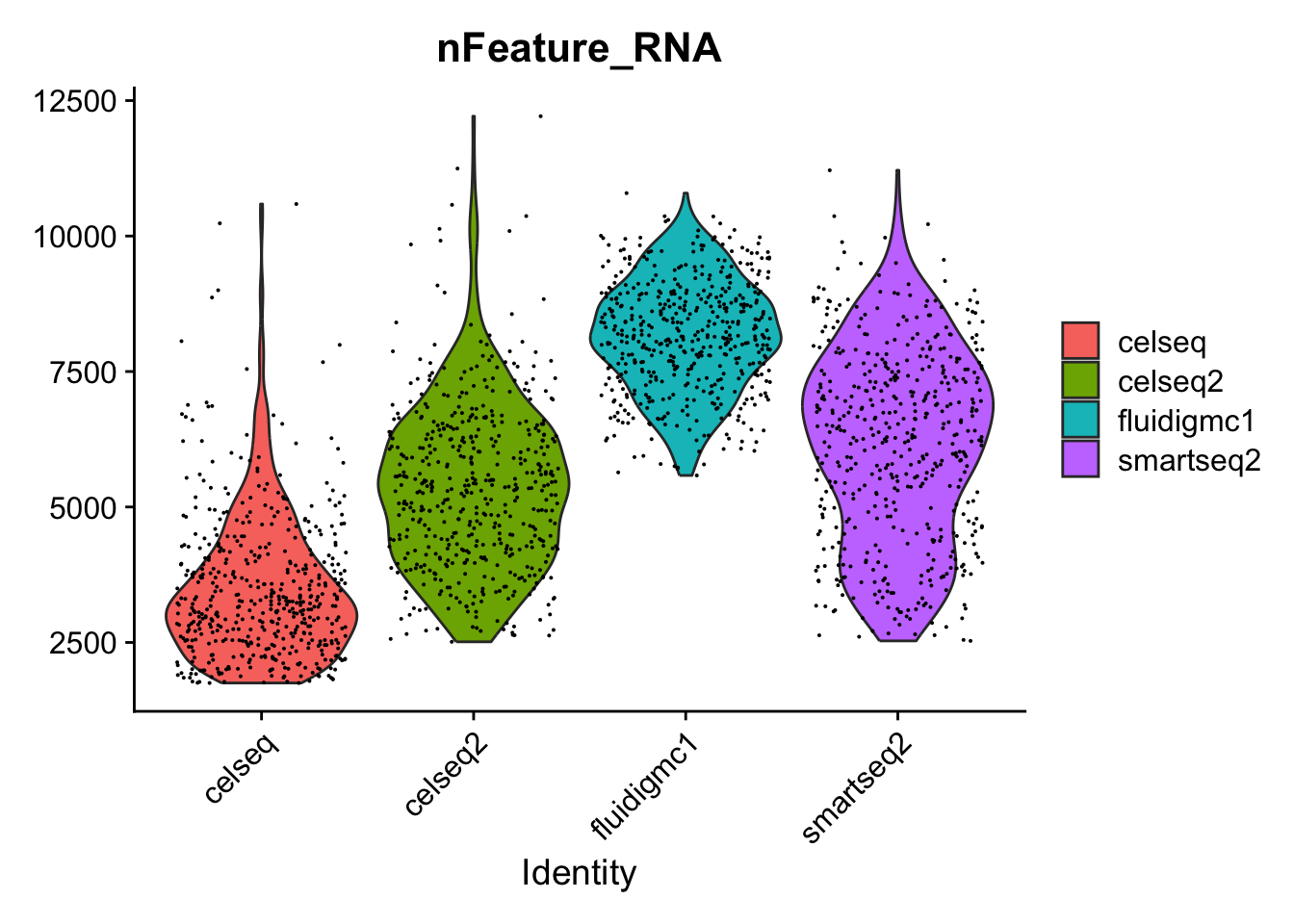
Four different datasets are provided in the ~/Share/batch_correction/ directory. These datasets were collected using different single cell RNA-seq technologies.

Question

Import the four datasets into R. What is the size and sparsity of each dataset?

R
celseq.data <- read.table("~/Share/batch_correction/pancreas_multi_celseq_expression_matrix.txt.gz")
celseq2.data <- read.table("~/Share/batch_correction/pancreas_multi_celseq2_expression_matrix.txt.gz")
fluidigmc1.data <- read.table("~/Share/batch_correction/pancreas_multi_fluidigmc1_expression_matrix.txt.gz")
smartseq2.data <- read.table("~/Share/batch_correction/pancreas_multi_smartseq2_expression_matrix.txt.gz")

Coerce each dataset to a sparse matrix for efficiency.

R
# Convert to sparse matrices for efficiency
library(Matrix)
celseq.data <- as(as.matrix(celseq.data), "dgCMatrix")
celseq2.data <- as(as.matrix(celseq2.data), "dgCMatrix")
fluidigmc1.data <- as(as.matrix(fluidigmc1.data), "dgCMatrix")
smartseq2.data <- as(as.matrix(smartseq2.data), "dgCMatrix")

11.2 Analyze each pancreas dataset without batch correction

We will first analyze each dataset separately to see if there are any differences between the datasets.

Question

What is the size of each single cell RNA-seq dataset?

Briefly describe the technology used to collect each dataset.

Which datasets do you expect to be different and which do you expect to be similar?

R
dim(celseq.data)
[1] 20148  1728
dim(celseq2.data)
[1] 19140  3072
dim(fluidigmc1.data)
[1] 25463   638
dim(smartseq2.data)
[1] 26179  3514
Question

Create a Seurat object for each dataset, and look at the distributions of number of genes per cell.

Loading required package: SeuratObject
Loading required package: sp
'SeuratObject' was built under R 4.4.0 but the current version is 4.4.1; it is recomended that you reinstall 'SeuratObject' as the ABI for R may have changed
'SeuratObject' was built with package 'Matrix' 1.7.0 but the current version is 1.7.1; it is recomended that you reinstall 'SeuratObject' as the ABI for 'Matrix' may have changed

Attaching package: 'SeuratObject'
The following objects are masked from 'package:base':

    intersect, t
# CEL-Seq (https://www.cell.com/cell-reports/fulltext/S2211-1247(12)00228-8)
celseq <- CreateSeuratObject(counts = celseq.data)
VlnPlot(celseq, "nFeature_RNA")
Warning: Default search for "data" layer in "RNA" assay yielded no results; utilizing "counts" layer instead.

# CEL-Seq2 https://www.cell.com/molecular-cell/fulltext/S1097-2765(09)00641-8
celseq2 <- CreateSeuratObject(counts = celseq2.data)
Warning: Feature names cannot have underscores ('_'), replacing with dashes ('-')
VlnPlot(celseq2, "nFeature_RNA")
Warning: Default search for "data" layer in "RNA" assay yielded no results; utilizing "counts" layer instead.

# Fluidigm C1
fluidigmc1 <- CreateSeuratObject(counts = fluidigmc1.data)
Warning: Feature names cannot have underscores ('_'), replacing with dashes ('-')
VlnPlot(fluidigmc1, "nFeature_RNA")
Warning: Default search for "data" layer in "RNA" assay yielded no results; utilizing "counts" layer instead.

# SMART-Seq2
smartseq2 <- CreateSeuratObject(counts = smartseq2.data)
Warning: Feature names cannot have underscores ('_'), replacing with dashes ('-')
VlnPlot(smartseq2, "nFeature_RNA")
Warning: Default search for "data" layer in "RNA" assay yielded no results; utilizing "counts" layer instead.

Now we will subset the data to remove cells with low gene counts and normalize the data.

Question

Subset the data to remove cells with:

  • fewer than 1750 genes for CEL-Seq;
  • fewer than 2500 genes for CEL-Seq2;
  • fewer than 2500 genes for SMART-Seq2.
R
celseq <- subset(celseq, subset = nFeature_RNA > 1750)
VlnPlot(celseq, "nFeature_RNA")
Warning: Default search for "data" layer in "RNA" assay yielded no results; utilizing "counts" layer instead.

celseq2 <- subset(celseq2, subset = nFeature_RNA > 2500)
VlnPlot(celseq2, "nFeature_RNA")
Warning: Default search for "data" layer in "RNA" assay yielded no results; utilizing "counts" layer instead.

smartseq2 <- subset(smartseq2, subset = nFeature_RNA > 2500)
VlnPlot(smartseq2, "nFeature_RNA")
Warning: Default search for "data" layer in "RNA" assay yielded no results; utilizing "counts" layer instead.

Now we will subsample each dataset to only have 500 cells. This is to speed up subsequent analyses. Often when we are setting up our analysis, we work with a subset of the data to make iteration across analysis decisions faster, and once we have finalized how we want to do the analysis, we work with the full dataset.

Question
  • Within metadata dataframe, save what technology each dataset was generated with.
  • Randomly subsample each full dataset to 500 cells.
R
celseq[["tech"]] <- "celseq"
celseq2[["tech"]] <- "celseq2"
fluidigmc1[["tech"]] <- "fluidigmc1"
smartseq2[["tech"]] <- "smartseq2"
Idents(celseq) <- "tech"
Idents(celseq2) <- "tech"
Idents(fluidigmc1) <- "tech"
Idents(smartseq2) <- "tech"

# This code sub-samples the data in order to speed up calculations and not use too much memory.
celseq <- subset(celseq, downsample = 500, seed = 1)
celseq2 <- subset(celseq2, downsample = 500, seed = 1)
fluidigmc1 <- subset(fluidigmc1, downsample = 500, seed = 1)
smartseq2 <- subset(smartseq2, downsample = 500, seed = 1)

11.3 Cluster pancreatic datasets without batch correction

We will first merge all the cells from the four different experiments together, and cluster all the pancreatic islet datasets to see whether there is a batch effect.

Question

Merge the datasets into a single Seurat object.

R
# Merge Seurat objects. Original sample identities are stored in gcdata[["tech"]].
# Cell names will now have the format tech_cellID (smartseq2_cell1...)
add.cell.ids <- c("celseq", "celseq2", "fluidigmc1", "smartseq2")
gcdata <- merge(x = celseq, y = list(celseq2, fluidigmc1, smartseq2), add.cell.ids = add.cell.ids, merge.data = FALSE)

# Examine gcdata. Notice that there are now 4 counts layers, one layer for each technology.
gcdata
An object of class Seurat 
33633 features across 2000 samples within 1 assay 
Active assay: RNA (33633 features, 0 variable features)
 4 layers present: counts.1, counts.2, counts.3, counts.4
VlnPlot(gcdata, "nFeature_RNA", group.by = "tech")
Warning: Default search for "data" layer in "RNA" assay yielded no results; utilizing "counts" layer instead.

After merging, we normalize the data with LogNormalize method, and identify the 2000 most variable genes for each dataset, using the vst approach. Then we scale the data using ScaleData.

Question

What is the difference between SelectIntegrationFeatures and FindVariableFeatures in Seurat? Take a look at the documentation for both functions.

Run NormalizeData, FindVariableFeatures, and ScaleData on the merged dataset.

R
gcdata <- NormalizeData(gcdata, normalization.method = "LogNormalize", scale.factor = 10000)
Normalizing layer: counts.1
Normalizing layer: counts.2
Normalizing layer: counts.3
Normalizing layer: counts.4
gcdata <- FindVariableFeatures(gcdata, nfeatures = 2000, verbose = TRUE, selection.method = "vst")
Finding variable features for layer counts.1
Finding variable features for layer counts.2
Finding variable features for layer counts.3
Finding variable features for layer counts.4
gcdata <- ScaleData(gcdata, features = VariableFeatures(gcdata))
Centering and scaling data matrix

Now that data is merged, normalized, and scaled, we will perform principal component analysis (PCA) and visualize the data.

Question

Do PCA on data including only the variable genes.

R
gcdata <- RunPCA(gcdata, features = VariableFeatures(gcdata), npcs = 40, ndims.print = 1:5, nfeatures.print = 5)
PC_ 1 
Positive:  CHGB, SCG2, ABCC8, PAM, CHGA 
Negative:  IFITM3, ZFP36L1, TACSTD2, ANXA4, LGALS3 
PC_ 2 
Positive:  SPARC, COL1A2, COL3A1, COL15A1, COL5A1 
Negative:  KRT8, CLDN4, ELF3, GATM, CFB 
PC_ 3 
Positive:  CCDC142, RAMP2-AS1, L2HGDH, NLRP12, TMEM212 
Negative:  PDGFRB, COL15A1, SFRP2, COL1A2, BGN 
PC_ 4 
Positive:  CPA2, CTRC, CTRB1, CPA1, CTRB2 
Negative:  CFTR, AQP1, VTCN1, SPP1, KRT19 
PC_ 5 
Positive:  TM4SF4, GC, IRX2, ARX, CRYBA2 
Negative:  PFKFB2, HADH, INS, IAPP, ADCYAP1 

Color the PCA biplot by the scRNA-seq technology.

R
DimPlot(gcdata, reduction = "pca", dims = c(1, 2), group.by = "tech")

Now we will cluster the cells and visualize the clusters in reduced dimensional space.

Question
  • Find the k=20 nearest neighbors for each cell in the PCA space, using the first 20 principal components.
  • Cluster the cells.
  • Perform UMAP embedding and visualize clustering results in 2D.
R
# Cluster the cells using the first twenty principal components.
gcdata <- FindNeighbors(gcdata, reduction = "pca", dims = 1:20, k.param = 20)
Computing nearest neighbor graph
Computing SNN
gcdata <- FindClusters(gcdata, resolution = 0.8, algorithm = 1, random.seed = 100)
Modularity Optimizer version 1.3.0 by Ludo Waltman and Nees Jan van Eck

Number of nodes: 2000
Number of edges: 59992

Running Louvain algorithm...
Maximum modularity in 10 random starts: 0.9181
Number of communities: 16
Elapsed time: 0 seconds
# Create a UMAP visualization. 
gcdata <- RunUMAP(gcdata, dims = 1:20, reduction = "pca", n.neighbors = 15, min.dist = 0.5, spread = 1, metric = "euclidean", seed.use = 1)  
Warning: The default method for RunUMAP has changed from calling Python UMAP via reticulate to the R-native UWOT using the cosine metric
To use Python UMAP via reticulate, set umap.method to 'umap-learn' and metric to 'correlation'
This message will be shown once per session
23:08:01 UMAP embedding parameters a = 0.583 b = 1.334
23:08:01 Read 2000 rows and found 20 numeric columns
23:08:01 Using FNN for neighbor search, n_neighbors = 15
23:08:01 Commencing smooth kNN distance calibration using 1 thread with target n_neighbors = 15
23:08:01 Initializing from normalized Laplacian + noise (using RSpectra)
23:08:01 Commencing optimization for 500 epochs, with 39324 positive edges
23:08:03 Optimization finished
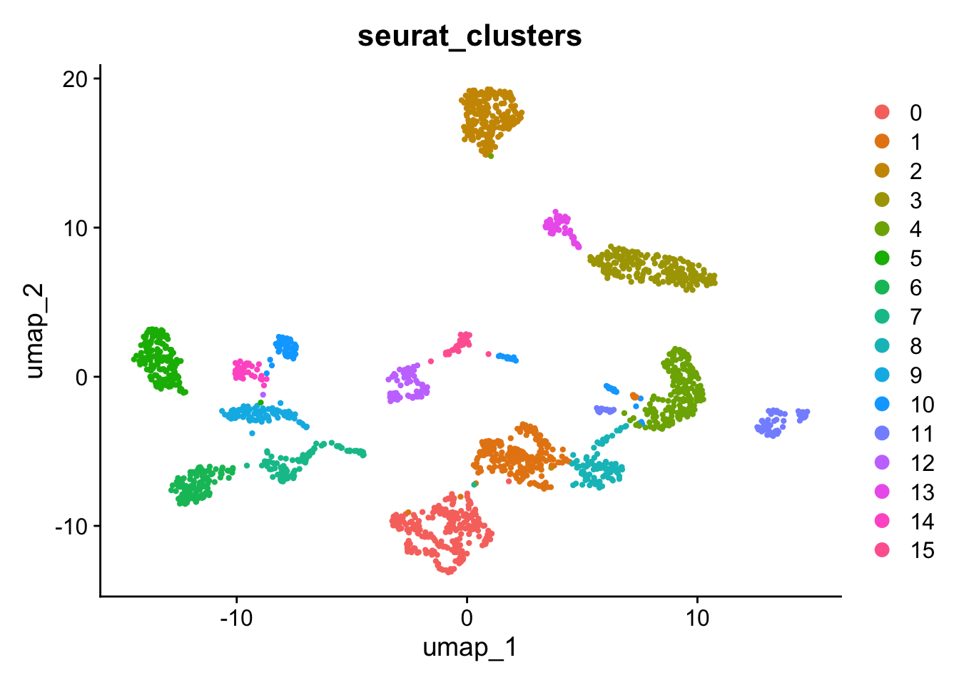
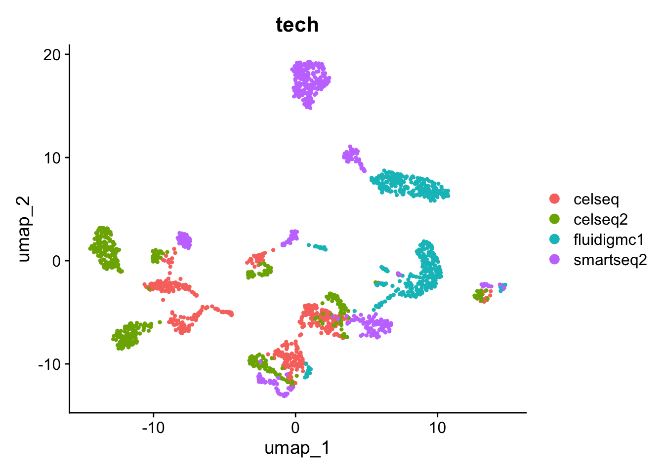
# Visualize the Leiden clustering and the batches on the UMAP. 
# Remember, the clustering is stored in @meta.data in column seurat_clusters and the technology is
# stored in the column tech. Remember you can also use DimPlot
DimPlot(gcdata, reduction = "umap", group.by = "seurat_clusters")

DimPlot(gcdata, reduction = "umap", group.by = "tech")

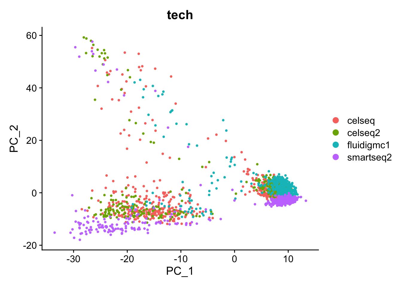
Are you surprised by the results? Compare to your expectations from the PC biplot of PC1 vs PC2.

What explains these results?

We can assess the quality of the clustering by calculating the adjusted rand index (ARI) between the technology and the cluster labels. This goes between 0 (completely dissimilar clustering) to 1 (identical clustering). The adjustment corrects for chance grouping between cluster elements.

Loading required package: maps
Loading required package: shapefiles
Loading required package: foreign

Attaching package: 'shapefiles'
The following objects are masked from 'package:foreign':

    read.dbf, write.dbf
ari <- dplyr::select(gcdata[[]], tech, seurat_clusters)
ari$tech <- plyr::mapvalues(ari$tech, from = c("celseq", "celseq2", "fluidigmc1", "smartseq2"), to = c(0, 1, 2, 3))
adj.rand.index(as.numeric(ari$tech), as.numeric(ari$seurat_clusters))
[1] 0.78898

11.4 Batch correction: canonical correlation analysis (CCA)+ mutual nearest neighbors (MNN)

We will now use Seurat to see to what extent it can remove potential batch effects.

The first piece of code will identify variable genes that are highly variable in at least 2/4 datasets. We will use these variable genes in our batch correction.

Why would we implement such a requirement?

Question

The integration workflow in Seurat requires the identification of variable genes that are variable across most samples. Use the IntegrateLayers function, with the CCAIntegration method, to identify anchors on the 4 pancreatic islet datasets, commonly shared variable genes across samples, and integrate samples.

R
gcdata <- IntegrateLayers(object = gcdata, method = CCAIntegration, orig.reduction = "pca", new.reduction = "integrated.cca", verbose = FALSE)

Now that the integration anchors have been used to integrate multiple datasets, we will perform the same clustering analysis as before.

Question
  • Perform analysis in the new integrated.cca dimensional reduction space.
  • Cluster the cells.
  • Perform UMAP embedding and visualize clustering results in 2D.
R
# Re-join the four layers after integration.
gcdata[["RNA"]] <- JoinLayers(gcdata[["RNA"]])

# Clustering
gcdata <- FindNeighbors(gcdata, reduction = "integrated.cca", dims = 1:20, k.param = 20)
Computing nearest neighbor graph
Computing SNN
gcdata <- FindClusters(gcdata, resolution = 0.8, algorithm = 1, random.seed = 100)
Modularity Optimizer version 1.3.0 by Ludo Waltman and Nees Jan van Eck

Number of nodes: 2000
Number of edges: 85037

Running Louvain algorithm...
Maximum modularity in 10 random starts: 0.8427
Number of communities: 9
Elapsed time: 0 seconds
# UMAP
gcdata <- RunUMAP(gcdata, dims = 1:30, reduction = "integrated.cca", n.neighbors = 15, min.dist = 0.5, spread = 1, metric = "euclidean", seed.use = 1)
23:08:16 UMAP embedding parameters a = 0.583 b = 1.334
23:08:16 Read 2000 rows and found 30 numeric columns
23:08:16 Using FNN for neighbor search, n_neighbors = 15
23:08:16 Commencing smooth kNN distance calibration using 1 thread with target n_neighbors = 15
23:08:16 Initializing from normalized Laplacian + noise (using RSpectra)
23:08:16 Commencing optimization for 500 epochs, with 44152 positive edges
23:08:18 Optimization finished
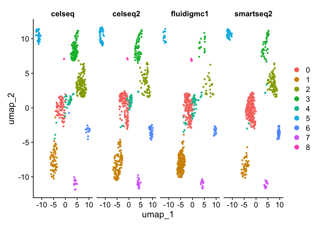
# Visualize the Louvain clustering and the batches on the UMAP. 
p1 <- DimPlot(gcdata, reduction = "umap", group.by = "seurat_clusters")
p2 <- DimPlot(gcdata, reduction = "umap", group.by = "tech")
p1 + p2

# Individually Visualize each technology dataset.
DimPlot(gcdata, reduction = "umap", split.by = "tech")

Let’s look again to see how the adjusted rand index changed compared to using no batch correction.

R
ari <- dplyr::select(gcdata[[]], tech, seurat_clusters)
ari$tech <- plyr::mapvalues(ari$tech, from = c("celseq", "celseq2", "fluidigmc1", "smartseq2"), to = c(0, 1, 2, 3))
adj.rand.index(as.numeric(ari$tech), as.numeric(ari$seurat_clusters))
[1] 0.29663

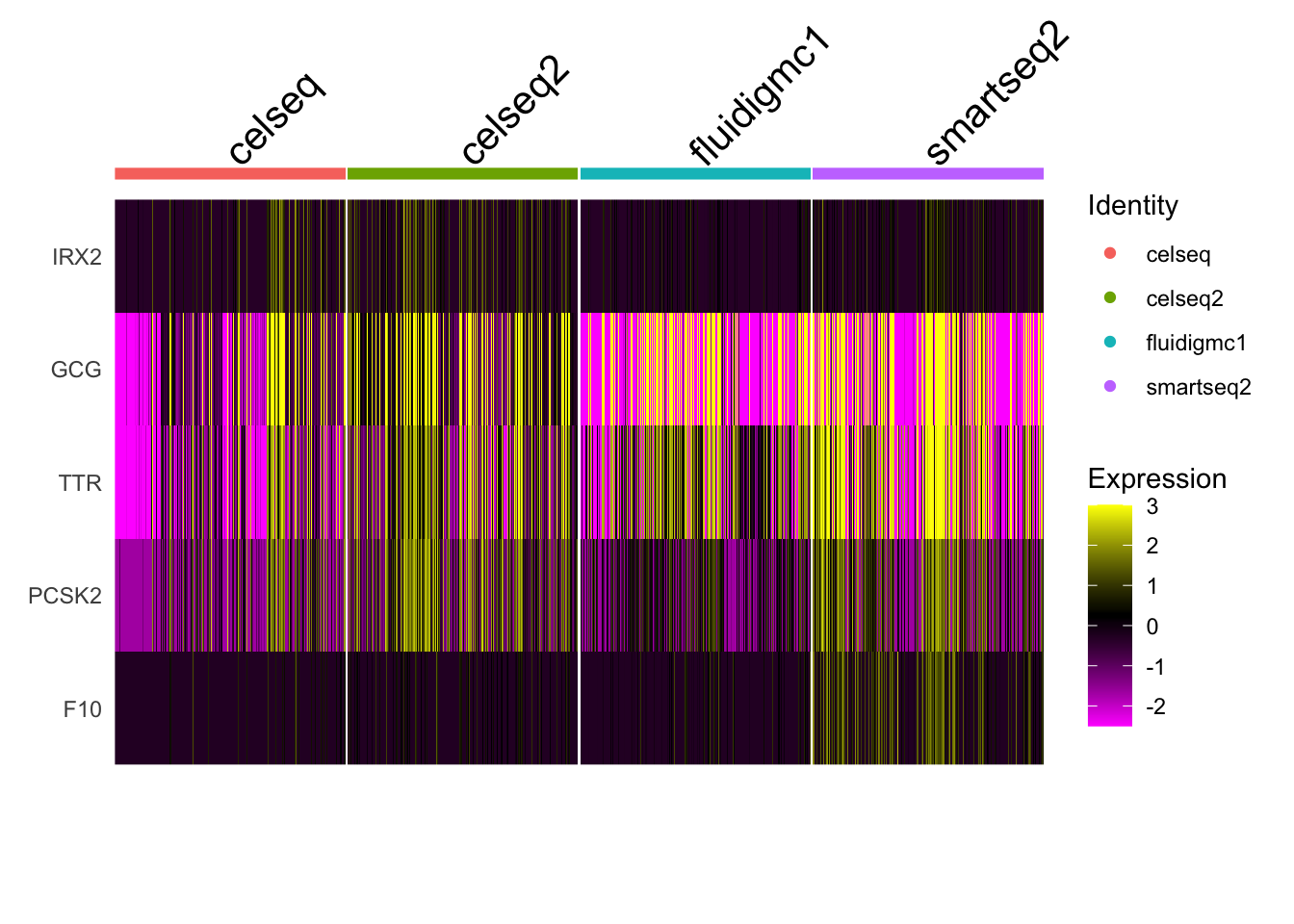
11.4.1 Differential gene expression and visualization

We can also identify conserved marker genes across the batches. Differential gene expression is done across each batch, and the p-values are combined. (requires metap package installation). Note that we use the original expression data in all visualization and DE tests. We should never use values from the integrated data in DE tests, as they violate assumptions of independence among samples that are required for DE tests!

R
markers <- FindConservedMarkers(gcdata, ident.1 = 0, grouping.var = "tech", assay = "RNA", print.bar = TRUE)
Testing group celseq: (0) vs (3, 2, 1, 4, 5, 7, 6, 8)
For a (much!) faster implementation of the Wilcoxon Rank Sum Test,
(default method for FindMarkers) please install the presto package
--------------------------------------------
install.packages('devtools')
devtools::install_github('immunogenomics/presto')
--------------------------------------------
After installation of presto, Seurat will automatically use the more 
efficient implementation (no further action necessary).
This message will be shown once per session
Testing group celseq2: (0) vs (2, 3, 6, 7, 1, 4, 5, 8)
Testing group fluidigmc1: (0) vs (2, 1, 4, 7, 3, 6, 5, 8)
Testing group smartseq2: (0) vs (1, 5, 4, 6, 3, 2, 7)
head(markers)
       celseq_p_val celseq_avg_log2FC celseq_pct.1 celseq_pct.2 celseq_p_val_adj celseq2_p_val celseq2_avg_log2FC celseq2_pct.1 celseq2_pct.2 celseq2_p_val_adj fluidigmc1_p_val fluidigmc1_avg_log2FC
IRX2     1.8435e-64            4.3477        0.921        0.090       6.2002e-60    5.6331e-52             2.5731         0.974         0.233        1.8946e-47       9.5921e-58                2.9715
GCG      1.5874e-38            4.4595        0.987        0.833       5.3389e-34    1.6633e-48             2.9664         1.000         1.000        5.5941e-44       1.6438e-62                3.8328
TTR      3.7735e-40            4.0309        0.987        0.851       1.2691e-35    2.1670e-49             2.5407         1.000         1.000        7.2884e-45       6.0723e-56                2.5704
PCSK2    1.4578e-42            3.5741        0.987        0.495       4.9030e-38    1.3960e-43             1.9711         1.000         0.938        4.6952e-39       2.1342e-32                1.5479
F10      2.7709e-25            3.8108        0.447        0.050       9.3193e-21    3.5541e-35             2.4476         0.728         0.142        1.1954e-30       1.8710e-41                2.1900
CRYBA2   4.4204e-51            4.4266        0.974        0.250       1.4867e-46    1.8107e-40             2.3144         0.921         0.308        6.0901e-36       2.3536e-32                2.2265
       fluidigmc1_pct.1 fluidigmc1_pct.2 fluidigmc1_p_val_adj smartseq2_p_val smartseq2_avg_log2FC smartseq2_pct.1 smartseq2_pct.2 smartseq2_p_val_adj   max_pval minimump_p_val
IRX2              0.903            0.149           3.2261e-53      2.6683e-79               4.6777           0.932           0.079          8.9741e-75 5.6331e-52     1.0673e-78
GCG               1.000            0.961           5.5287e-58      1.6148e-78               5.7615           1.000           0.979          5.4311e-74 1.5874e-38     6.4592e-78
TTR               1.000            0.927           2.0423e-51      3.3401e-78               3.9099           1.000           0.986          1.1234e-73 3.7735e-40     1.3360e-77
PCSK2             1.000            0.860           7.1781e-28      1.4128e-70               2.8320           1.000           0.664          4.7516e-66 2.1342e-32     5.6512e-70
F10               0.764            0.132           6.2926e-37      2.7110e-69               3.5655           0.968           0.304          9.1180e-65 2.7709e-25     1.0844e-68
CRYBA2            0.944            0.449           7.9158e-28      4.4701e-69               4.5109           0.986           0.546          1.5034e-64 2.3536e-32     1.7880e-68
Question

Visualize the expression of the first 5 marker genes on UMAP across the different batches using DoHeatmap.

R
gcdata <- ScaleData(gcdata, features = rownames(gcdata), do.center = T, do.scale = F)
Centering data matrix
Warning: Different features in new layer data than already exists for scale.data
DoHeatmap(gcdata, features = rownames(markers)[1:5], group.by = "tech", disp.max = 3)

Check the expression of some known marker genes for pancreatic cells (see the Human pancreas cell atlas).

R
genes <- c("GCG", "INS", "SST", "PPY", "PRSS1", "KRT19", "PECAM1", "COL1A1")
FeaturePlot(gcdata, genes, ncol = 4)

11.5 Batch correction: integrative non-negative matrix factorization (NMF)

Here we use integrative non-negative matrix factorization (NMF/LIGER) to see to what extent it can remove potential batch effects.

The important parameters in the batch correction are the number of factors (k), the penalty parameter (lambda), and the clustering resolution. The number of factors sets the number of factors (consisting of shared and dataset-specific factors) used in factorizing the matrix. The penalty parameter sets the balance between factors shared across the batches and factors specific to the individual batches. The default setting of lambda=5.0 is usually used by the Macosko lab. Resolution=1.0 is used in the Louvain clustering of the shared neighbor factors that have been quantile normalized.

R
ob.list <- list("celseq" = celseq, "celseq2" = celseq2, "fluidigmc1" = fluidigmc1, "smartseq2" = smartseq2)

# Create a LIGER object with raw counts data from each batch.
library(rliger)
Package `rliger` has been updated massively since version 1.99.0, including the object structure which is not compatible with old versions.

We recommand you backup your old analysis before overwriting any existing result.

`readLiger()` is provided for reading an RDS file storing an old object and it converts the object to the up-to-date structure.
data.liger <- createLiger(sapply(ob.list, function(data) LayerData(data[['RNA']], 'counts')[, colnames(data)]))
ℹ calculating QC for dataset "celseq"
✔ calculating QC for dataset "celseq" ... done
ℹ calculating QC for dataset "celseq2"
✔ calculating QC for dataset "celseq2" ... done
ℹ calculating QC for dataset "fluidigmc1"
✔ calculating QC for dataset "fluidigmc1" ... done
ℹ calculating QC for dataset "smartseq2"
✔ calculating QC for dataset "smartseq2" ... done
ℹ Removing missing in dataset: "celseq"
ℹ Removing missing in dataset: "celseq2"
ℹ Removing missing in dataset: "fluidigmc1"
ℹ Removing missing in dataset: "smartseq2"
# Normalize gene expression for each batch.
data.liger <- rliger::normalize(data.liger)
ℹ Normalizing datasets "celseq"
ℹ Normalizing datasets "celseq2"
ℹ Normalizing datasets "fluidigmc1"
ℹ Normalizing datasets "smartseq2"
✔ Normalizing datasets "smartseq2" ... done
ℹ Normalizing datasets "fluidigmc1"
✔ Normalizing datasets "fluidigmc1" ... done

ℹ Normalizing datasets "celseq2"
✔ Normalizing datasets "celseq2" ... done

ℹ Normalizing datasets "celseq"
✔ Normalizing datasets "celseq" ... done
# Find variable genes for LIGER analysis. Identify variable genes that are variable across most samples.
var.genes <- SelectIntegrationFeatures(ob.list, nfeatures = 2000, verbose = TRUE, fvf.nfeatures = 2000, selection.method = "vst")
No variable features found for object1 in the object.list. Running FindVariableFeatures ...
Finding variable features for layer counts
No variable features found for object2 in the object.list. Running FindVariableFeatures ...
Finding variable features for layer counts
No variable features found for object3 in the object.list. Running FindVariableFeatures ...
Finding variable features for layer counts
No variable features found for object4 in the object.list. Running FindVariableFeatures ...
Finding variable features for layer counts
data.liger@varFeatures <- var.genes
print(length(varFeatures(data.liger)))
[1] 2000
Question

Scale the gene expression across the datasets.

Why does LIGER not center the data?

Hint: think about the use of non-negative matrix factorization and the constraints that this imposes.

R
data.liger <- scaleNotCenter(data.liger)

Next, we will run the integrative non-negative matrix factorization.

Question

Use the runIntegration function to perform the integrative non-negative matrix factorization.

R
data.liger <- runIntegration(data.liger, k = 30)

What do matrices H, V, and W represent, and what are their dimensions?

R
dim(getMatrix(data.liger, "H")$celseq)
dim(getMatrix(data.liger, "V")$celseq)
dim(getMatrix(data.liger, "W"))

Next, do normalization and clustering of cells in shared nearest factor space.

Question

Do quantile normalization, cluster quantile normalized data

R
data.liger <- quantileNorm(data.liger, resolution = 1)
data.liger <- runCluster(data.liger)

What are the dimensions of H.norm. What does this represent?

R
dim(getMatrix(data.liger, "H.norm"))

Let’s see what the liger data looks like mapped onto a UMAP visualization.

Question

Run UMAP on the quantile normalized data and visualize the clusters.

R
data.liger <- runUMAP(data.liger, n_neighbors = 15, min_dist = 0.5)
p <- plotByDatasetAndCluster(data.liger) 
p

clusterUmapList <- plotClusterDimRed(data.liger, splitBy = "dataset", title = names(data.liger))
plot_grid(plotlist = c(clusterUmapList), align = "hv")

Finally, let’s look at the adjusted rand index between the clusters and technology, and also the genes that load the factors used in data integration.

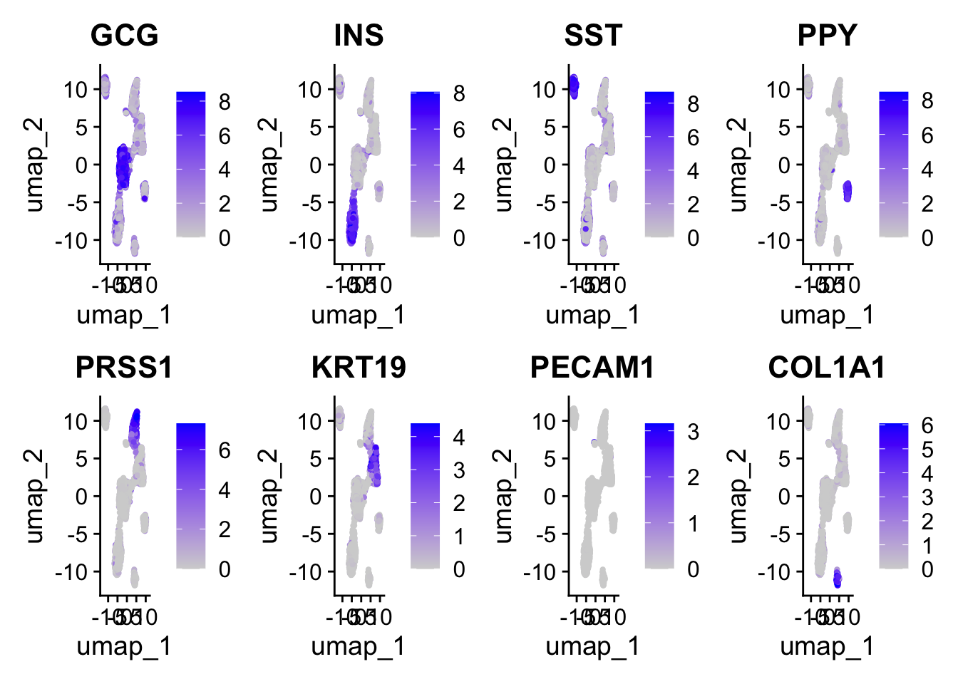
# Let's look to see how the adjusted rand index changed compared to using no batch correction.
tech <- cellMeta(data.liger)$dataset
clusters <- cellMeta(data.liger)$leiden_cluster
ari <- data.frame("tech" = tech, "clusters" = clusters)
ari$tech <- plyr::mapvalues(ari$tech, from = c("celseq", "celseq2", "fluidigmc1", "smartseq2"), to = c(0, 1, 2, 3))
adj.rand.index(as.numeric(ari$tech), as.numeric(ari$clusters))

# Identify shared and batch-specific marker genes from liger factorization.
# Use the getFactorMarkers function and choose 2 datasets.
# Then plot some genes of interest using plotGene functions.
markers <- getFactorMarkers(data.liger, dataset1 = "celseq2", dataset2 = "smartseq2")
plotGeneDimRed(data.liger, features = "INS")

# Look at factor loadings in factor 9, celseq2 vs smartseq2.
plotGeneLoadings(data.liger, markerTable = markers, useFactor = 9)

11.6 Additional exploration

11.6.1 Regressing out unwanted covariates

Learn how to regress out different technical covariates (number of UMIs, number of genes, percent mitochondrial reads) by studying Seurat’s PBMC tutorial and the ScaleData() function.

11.6.2 kBET

Within your RStudio session, install k-nearest neighbour batch effect test and learn how to use its functionality to quantify batch effects in the pancreatic data.

11.7 Acknowledgements

This document builds off a tutorial from the Seurat website and a tutorial from the LIGER website.

11.8 Session info

─ Session info ───────────────────────────────────────────────────────────────────────────────────────────────────────────────────────────────────────────────────────────────────────────────────────
 setting  value
 version  R version 4.4.1 (2024-06-14)
 os       macOS Sonoma 14.6.1
 system   aarch64, darwin20
 ui       X11
 language (EN)
 collate  en_US.UTF-8
 ctype    en_US.UTF-8
 tz       Europe/Paris
 date     2024-11-06
 pandoc   2.19.2 @ /opt/homebrew/bin/ (via rmarkdown)

─ Packages ───────────────────────────────────────────────────────────────────────────────────────────────────────────────────────────────────────────────────────────────────────────────────────────
 package          * version    date (UTC) lib source
 abind              1.4-8      2024-09-12 [1] CRAN (R 4.4.1)
 beeswarm           0.4.0      2021-06-01 [1] CRAN (R 4.4.0)
 Biobase            2.64.0     2024-04-30 [1] Bioconduc~
 BiocGenerics       0.50.0     2024-04-30 [1] Bioconduc~
 cachem             1.1.0      2024-05-16 [1] CRAN (R 4.4.0)
 cli                3.6.3      2024-06-21 [1] CRAN (R 4.4.0)
 cluster            2.1.6      2023-12-01 [1] CRAN (R 4.4.1)
 codetools          0.2-20     2024-03-31 [1] CRAN (R 4.4.1)
 colorspace         2.1-1      2024-07-26 [1] CRAN (R 4.4.0)
 cowplot            1.1.3      2024-01-22 [1] CRAN (R 4.4.0)
 data.table         1.16.2     2024-10-10 [1] CRAN (R 4.4.1)
 deldir             2.0-4      2024-02-28 [1] CRAN (R 4.4.0)
 devtools           2.4.5      2022-10-11 [1] CRAN (R 4.4.0)
 digest             0.6.37     2024-08-19 [1] CRAN (R 4.4.1)
 dotCall64          1.2        2024-10-04 [1] CRAN (R 4.4.1)
 dplyr              1.1.4      2023-11-17 [1] CRAN (R 4.4.0)
 ellipsis           0.3.2      2021-04-29 [1] CRAN (R 4.4.0)
 evaluate           1.0.1      2024-10-10 [1] CRAN (R 4.4.1)
 fansi              1.0.6      2023-12-08 [1] CRAN (R 4.4.0)
 farver             2.1.2      2024-05-13 [1] CRAN (R 4.4.0)
 fastDummies        1.7.4      2024-08-16 [1] CRAN (R 4.4.0)
 fastmap            1.2.0      2024-05-15 [1] CRAN (R 4.4.0)
 fitdistrplus       1.2-1      2024-07-12 [1] CRAN (R 4.4.0)
 FNN                1.1.4.1    2024-09-22 [1] CRAN (R 4.4.1)
 foreign          * 0.8-86     2023-11-28 [1] CRAN (R 4.4.1)
 fossil           * 0.4.0      2020-03-23 [1] CRAN (R 4.4.0)
 fs                 1.6.4      2024-04-25 [1] CRAN (R 4.4.0)
 future             1.34.0     2024-07-29 [1] CRAN (R 4.4.0)
 future.apply       1.11.3     2024-10-27 [1] CRAN (R 4.4.1)
 generics           0.1.3      2022-07-05 [1] CRAN (R 4.4.0)
 ggbeeswarm         0.7.2      2023-04-29 [1] CRAN (R 4.4.0)
 ggplot2            3.5.1      2024-04-23 [1] CRAN (R 4.4.0)
 ggrastr            1.0.2      2023-06-01 [1] CRAN (R 4.4.0)
 ggrepel            0.9.6      2024-09-07 [1] CRAN (R 4.4.1)
 ggridges           0.5.6      2024-01-23 [1] CRAN (R 4.4.0)
 globals            0.16.3     2024-03-08 [1] CRAN (R 4.4.0)
 glue               1.8.0      2024-09-30 [1] CRAN (R 4.4.1)
 goftest            1.2-3      2021-10-07 [1] CRAN (R 4.4.0)
 gridExtra          2.3        2017-09-09 [1] CRAN (R 4.4.0)
 gtable             0.3.6      2024-10-25 [1] CRAN (R 4.4.1)
 htmltools          0.5.8.1    2024-04-04 [1] CRAN (R 4.4.0)
 htmlwidgets        1.6.4      2023-12-06 [1] CRAN (R 4.4.0)
 httpuv             1.6.15     2024-03-26 [1] CRAN (R 4.4.0)
 httr               1.4.7      2023-08-15 [1] CRAN (R 4.4.0)
 ica                1.0-3      2022-07-08 [1] CRAN (R 4.4.0)
 igraph             2.1.1      2024-10-19 [1] CRAN (R 4.4.1)
 irlba              2.3.5.1    2022-10-03 [1] CRAN (R 4.4.0)
 jsonlite           1.8.9      2024-09-20 [1] CRAN (R 4.4.1)
 KernSmooth         2.23-24    2024-05-17 [1] CRAN (R 4.4.1)
 knitr              1.48       2024-07-07 [1] CRAN (R 4.4.0)
 labeling           0.4.3      2023-08-29 [1] CRAN (R 4.4.0)
 later              1.3.2      2023-12-06 [1] CRAN (R 4.4.0)
 lattice            0.22-6     2024-03-20 [1] CRAN (R 4.4.1)
 lazyeval           0.2.2      2019-03-15 [1] CRAN (R 4.4.0)
 leiden             0.4.3.1    2023-11-17 [1] CRAN (R 4.4.0)
 lifecycle          1.0.4      2023-11-07 [1] CRAN (R 4.4.0)
 limma              3.60.6     2024-10-02 [1] Bioconduc~
 listenv            0.9.1      2024-01-29 [1] CRAN (R 4.4.0)
 lmtest             0.9-40     2022-03-21 [1] CRAN (R 4.4.0)
 magrittr           2.0.3      2022-03-30 [1] CRAN (R 4.4.0)
 maps             * 3.4.2      2023-12-15 [1] CRAN (R 4.4.0)
 MASS               7.3-60.2   2024-04-26 [1] CRAN (R 4.4.1)
 mathjaxr           1.6-0      2022-02-28 [1] CRAN (R 4.4.0)
 Matrix           * 1.7-1      2024-10-18 [1] CRAN (R 4.4.1)
 matrixStats        1.4.1      2024-09-08 [1] CRAN (R 4.4.1)
 memoise            2.0.1      2021-11-26 [1] CRAN (R 4.4.0)
 metap              1.11       2024-07-11 [1] CRAN (R 4.4.0)
 mime               0.12       2021-09-28 [1] CRAN (R 4.4.0)
 miniUI             0.1.1.1    2018-05-18 [1] CRAN (R 4.4.0)
 mnormt             2.1.1      2022-09-26 [1] CRAN (R 4.4.0)
 multcomp           1.4-26     2024-07-18 [1] CRAN (R 4.4.0)
 multtest           2.60.0     2024-04-30 [1] Bioconduc~
 munsell            0.5.1      2024-04-01 [1] CRAN (R 4.4.0)
 mutoss             0.1-13     2023-03-14 [1] CRAN (R 4.4.0)
 mvtnorm            1.3-1      2024-09-03 [1] CRAN (R 4.4.1)
 nlme               3.1-164    2023-11-27 [1] CRAN (R 4.4.1)
 numDeriv           2016.8-1.1 2019-06-06 [1] CRAN (R 4.4.0)
 parallelly         1.38.0     2024-07-27 [1] CRAN (R 4.4.0)
 patchwork          1.3.0      2024-09-16 [1] CRAN (R 4.4.1)
 pbapply            1.7-2      2023-06-27 [1] CRAN (R 4.4.0)
 pillar             1.9.0      2023-03-22 [1] CRAN (R 4.4.0)
 pkgbuild           1.4.5      2024-10-28 [1] CRAN (R 4.4.1)
 pkgconfig          2.0.3      2019-09-22 [1] CRAN (R 4.4.0)
 pkgload            1.4.0      2024-06-28 [1] CRAN (R 4.4.0)
 plotly             4.10.4     2024-01-13 [1] CRAN (R 4.4.0)
 plotrix            3.8-4      2023-11-10 [1] CRAN (R 4.4.0)
 plyr               1.8.9      2023-10-02 [1] CRAN (R 4.4.0)
 png                0.1-8      2022-11-29 [1] CRAN (R 4.4.0)
 polyclip           1.10-7     2024-07-23 [1] CRAN (R 4.4.0)
 profvis            0.4.0      2024-09-20 [1] CRAN (R 4.4.1)
 progressr          0.14.0     2023-08-10 [1] CRAN (R 4.4.0)
 promises           1.3.0      2024-04-05 [1] CRAN (R 4.4.0)
 purrr              1.0.2      2023-08-10 [1] CRAN (R 4.4.0)
 qqconf             1.3.2      2023-04-14 [1] CRAN (R 4.4.0)
 R6                 2.5.1      2021-08-19 [1] CRAN (R 4.4.0)
 RANN               2.6.2      2024-08-25 [1] CRAN (R 4.4.1)
 rbibutils          2.3        2024-10-04 [1] CRAN (R 4.4.1)
 RColorBrewer       1.1-3      2022-04-03 [1] CRAN (R 4.4.0)
 Rcpp               1.0.13     2024-07-17 [1] CRAN (R 4.4.0)
 RcppAnnoy          0.0.22     2024-01-23 [1] CRAN (R 4.4.0)
 RcppHNSW           0.6.0      2024-02-04 [1] CRAN (R 4.4.0)
 Rdpack             2.6.1      2024-08-06 [1] CRAN (R 4.4.0)
 remotes            2.5.0      2024-03-17 [1] CRAN (R 4.4.0)
 reshape2           1.4.4      2020-04-09 [1] CRAN (R 4.4.0)
 reticulate         1.39.0     2024-09-05 [1] CRAN (R 4.4.1)
 rlang              1.1.4      2024-06-04 [1] CRAN (R 4.4.0)
 rliger           * 2.0.1      2024-04-04 [1] CRAN (R 4.4.0)
 rmarkdown          2.28       2024-08-17 [1] CRAN (R 4.4.0)
 ROCR               1.0-11     2020-05-02 [1] CRAN (R 4.4.0)
 RSpectra           0.16-2     2024-07-18 [1] CRAN (R 4.4.0)
 Rtsne              0.17       2023-12-07 [1] CRAN (R 4.4.0)
 S4Vectors          0.42.1     2024-07-03 [1] Bioconduc~
 sandwich           3.1-1      2024-09-15 [1] CRAN (R 4.4.1)
 scales             1.3.0      2023-11-28 [1] CRAN (R 4.4.0)
 scattermore        1.2        2023-06-12 [1] CRAN (R 4.4.0)
 sctransform        0.4.1      2023-10-19 [1] CRAN (R 4.4.0)
 sessioninfo        1.2.2      2021-12-06 [1] CRAN (R 4.4.0)
 Seurat           * 5.1.0      2024-05-10 [1] CRAN (R 4.4.0)
 SeuratObject     * 5.0.2      2024-05-08 [1] CRAN (R 4.4.0)
 shapefiles       * 0.7.2      2022-08-25 [1] CRAN (R 4.4.0)
 shiny              1.9.1      2024-08-01 [1] CRAN (R 4.4.0)
 sn                 2.1.1      2023-04-04 [1] CRAN (R 4.4.0)
 sp               * 2.1-4      2024-04-30 [1] CRAN (R 4.4.0)
 spam               2.11-0     2024-10-03 [1] CRAN (R 4.4.1)
 spatstat.data      3.1-2      2024-06-21 [1] CRAN (R 4.4.0)
 spatstat.explore   3.3-3      2024-10-22 [1] CRAN (R 4.4.1)
 spatstat.geom      3.3-3      2024-09-18 [1] CRAN (R 4.4.1)
 spatstat.random    3.3-2      2024-09-18 [1] CRAN (R 4.4.1)
 spatstat.sparse    3.1-0      2024-06-21 [1] CRAN (R 4.4.0)
 spatstat.univar    3.0-1      2024-09-05 [1] CRAN (R 4.4.1)
 spatstat.utils     3.1-0      2024-08-17 [1] CRAN (R 4.4.0)
 statmod            1.5.0      2023-01-06 [1] CRAN (R 4.4.0)
 stringi            1.8.4      2024-05-06 [1] CRAN (R 4.4.0)
 stringr            1.5.1      2023-11-14 [1] CRAN (R 4.4.0)
 survival           3.6-4      2024-04-24 [1] CRAN (R 4.4.1)
 tensor             1.5        2012-05-05 [1] CRAN (R 4.4.0)
 TFisher            0.2.0      2018-03-21 [1] CRAN (R 4.4.0)
 TH.data            1.1-2      2023-04-17 [1] CRAN (R 4.4.0)
 tibble             3.2.1      2023-03-20 [1] CRAN (R 4.4.0)
 tidyr              1.3.1      2024-01-24 [1] CRAN (R 4.4.0)
 tidyselect         1.2.1      2024-03-11 [1] CRAN (R 4.4.0)
 urlchecker         1.0.1      2021-11-30 [1] CRAN (R 4.4.0)
 usethis            3.0.0      2024-07-29 [1] CRAN (R 4.4.0)
 utf8               1.2.4      2023-10-22 [1] CRAN (R 4.4.0)
 uwot               0.2.2      2024-04-21 [1] CRAN (R 4.4.0)
 vctrs              0.6.5      2023-12-01 [1] CRAN (R 4.4.0)
 vipor              0.4.7      2023-12-18 [1] CRAN (R 4.4.0)
 viridisLite        0.4.2      2023-05-02 [1] CRAN (R 4.4.0)
 withr              3.0.2      2024-10-28 [1] CRAN (R 4.4.1)
 xfun               0.48       2024-10-03 [1] CRAN (R 4.4.1)
 xtable             1.8-4      2019-04-21 [1] CRAN (R 4.4.0)
 zoo                1.8-12     2023-04-13 [1] CRAN (R 4.4.0)

 [1] /Library/Frameworks/R.framework/Versions/4.4-arm64/Resources/library

──────────────────────────────────────────────────────────────────────────────────────────────────────────────────────────────────────────────────────────────────────────────────────────────────────