R
install.packages('mgcv')The estimated time for this lab is around 1h20.
R packages from different sources.R and Bioconductor.R and Bioconductor.Bioconductor and Seurat approaches to scRNAseq data analysis.R
“Hey, I’ve heard so many good things about this piece of software, it’s called ‘slingshot’? Heard of it? I really want to try it out on my dataset!!”
Or, in other words: “how do I install this or that brand new cutting-edge fancy package?”
R works with packages, available from different sources:
CRAN, the R developer team and official package provider: CRAN (which can probably win the title of “the worst webpage ever designed that survived until 2023”).Bioconductor, another package provider, with a primary focus on genomic-related packages: Bioconductor.GitHub.Let’s start by going over package installation.
Package help pages are available at different places, depending on their source. That being said, there is a place I like to go to easily find information related to most packages:
For instance, check out Revelio package help pages.
R and Bioconductor classesWhile CRAN is a repository of general-purpose packages, Bioconductor is the greatest source of analytical tools, data and workflows dedicated to genomic projects in R. Read more about Bioconductor to fully understand how it builds up on top of R general features, especially with the specific classes it introduces.
The two main concepts behind Bioconductor’s success are the non-redundant classes of objects it provides and their inter-operability. Huber et al., Nat. Methods 2015 summarizes it well.
tibble tables:tibbles are built on the fundamental data.frame objects. They follow “tidy” concepts, all gathered in a common tidyverse. This set of key concepts help general data investigation and data visualization through a set of associated packages such as ggplot2.
── Attaching core tidyverse packages ──────────────────────────────────────────────────────────────────────────────────────────────────────────────────────────────────────────────── tidyverse 2.0.0 ──
✔ dplyr     1.1.4     ✔ readr     2.1.5
✔ forcats   1.0.0     ✔ stringr   1.5.1
✔ ggplot2   3.5.1     ✔ tibble    3.2.1
✔ lubridate 1.9.3     ✔ tidyr     1.3.1
✔ purrr     1.0.2
── Conflicts ────────────────────────────────────────────────────────────────────────────────────────────────────────────────────────────────────────────────────────────────── tidyverse_conflicts() ──
✖ dplyr::filter() masks stats::filter()
✖ dplyr::lag()    masks stats::lag()
ℹ Use the conflicted package (<http://conflicted.r-lib.org/>) to force all conflicts to become errors# A tibble: 5 × 4
x y z class
<int> <dbl> <dbl> <chr>
1 1 1 2 a
2 2 1 5 a
3 3 1 10 b
4 4 1 17 b
5 5 1 26 c tibblestibbles can be created from text files (or Excel files) using the readr package (part of tidyverse)
Rows: 32738 Columns: 2
── Column specification ────────────────────────────────────────────────────────────────────────────────────────────────────────────────────────────────────────────────────────────────────────────────
Delimiter: "\t"
chr (2): ID, Symbol

ℹ Use `spec()` to retrieve the full column specification for this data.
ℹ Specify the column types or set `show_col_types = FALSE` to quiet this message.genes# A tibble: 32,738 × 2
ID Symbol
<chr> <chr>
1 ENSG00000243485 MIR1302-10
2 ENSG00000237613 FAM138A
3 ENSG00000186092 OR4F5
4 ENSG00000238009 RP11-34P13.7
5 ENSG00000239945 RP11-34P13.8
6 ENSG00000237683 AL627309.1
7 ENSG00000239906 RP11-34P13.14
8 ENSG00000241599 RP11-34P13.9
9 ENSG00000228463 AP006222.2
10 ENSG00000237094 RP4-669L17.10
# ℹ 32,728 more rowstibbles:tibbles can be readily “sliced” (i.e. selecting rows by number/name), “filtered” (i.e. selecting rows by condition) and columns can be “selected”. All these operations are performed using verbs (most of them provided by the dplyr package, part of tidyverse).
R
slice(genes, 1:4)# A tibble: 4 × 2
ID Symbol
<chr> <chr>
1 ENSG00000243485 MIR1302-10
2 ENSG00000237613 FAM138A
3 ENSG00000186092 OR4F5
4 ENSG00000238009 RP11-34P13.7filter(genes, Symbol == 'CCDC67')# A tibble: 1 × 2
ID Symbol
<chr> <chr>
1 ENSG00000165325 CCDC67# A tibble: 159 × 2
ID Symbol
<chr> <chr>
1 ENSG00000162592 CCDC27
2 ENSG00000160050 CCDC28B
3 ENSG00000186409 CCDC30
4 ENSG00000177868 CCDC23
5 ENSG00000159214 CCDC24
6 ENSG00000236624 CCDC163P
7 ENSG00000159588 CCDC17
8 ENSG00000122483 CCDC18
9 ENSG00000213085 CCDC19
10 ENSG00000117477 CCDC181
# ℹ 149 more rows# A tibble: 9 × 2
ID Symbol
<chr> <chr>
1 ENSG00000136710 CCDC115
2 ENSG00000183323 CCDC125
3 ENSG00000147419 CCDC25
4 ENSG00000149548 CCDC15
5 ENSG00000139537 CCDC65
6 ENSG00000151838 CCDC175
7 ENSG00000159625 CCDC135
8 ENSG00000160994 CCDC105
9 ENSG00000161609 CCDC155select(genes, 1)# A tibble: 32,738 × 1
ID
<chr>
1 ENSG00000243485
2 ENSG00000237613
3 ENSG00000186092
4 ENSG00000238009
5 ENSG00000239945
6 ENSG00000237683
7 ENSG00000239906
8 ENSG00000241599
9 ENSG00000228463
10 ENSG00000237094
# ℹ 32,728 more rowsselect(genes, ID)# A tibble: 32,738 × 1
ID
<chr>
1 ENSG00000243485
2 ENSG00000237613
3 ENSG00000186092
4 ENSG00000238009
5 ENSG00000239945
6 ENSG00000237683
7 ENSG00000239906
8 ENSG00000241599
9 ENSG00000228463
10 ENSG00000237094
# ℹ 32,728 more rows# A tibble: 32,738 × 1
Symbol
<chr>
1 MIR1302-10
2 FAM138A
3 OR4F5
4 RP11-34P13.7
5 RP11-34P13.8
6 AL627309.1
7 RP11-34P13.14
8 RP11-34P13.9
9 AP006222.2
10 RP4-669L17.10
# ℹ 32,728 more rowsColumns can also be quickly added/modified using the mutate verb.
# A tibble: 32,738 × 3
   ID              Symbol          chr
   <chr>           <chr>         <int>
 1 ENSG00000243485 MIR1302-10       15
 2 ENSG00000237613 FAM138A          18
 3 ENSG00000186092 OR4F5            21
 4 ENSG00000238009 RP11-34P13.7      1
 5 ENSG00000239945 RP11-34P13.8      9
 6 ENSG00000237683 AL627309.1       20
 7 ENSG00000239906 RP11-34P13.14    15
 8 ENSG00000241599 RP11-34P13.9     15
 9 ENSG00000228463 AP006222.2        4
10 ENSG00000237094 RP4-669L17.10    10
# ℹ 32,728 more rows|> pipe:Actions on tibbles can be piped as a chain with |>, just like | pipes stdout as the stdin of the next command in bash. In this case, the first argument is always the output of the previous function and is ommited. Because tidyverse functions generally return a modified version of the input, pipping works remarkably well in such context.
R
Rows: 32738 Columns: 2
── Column specification ────────────────────────────────────────────────────────────────────────────────────────────────────────────────────────────────────────────────────────────────────────────────
Delimiter: "\t"
chr (2): ID, Symbol

ℹ Use `spec()` to retrieve the full column specification for this data.
ℹ Specify the column types or set `show_col_types = FALSE` to quiet this message.
# A tibble: 3 × 1
ID
<chr>
1 ENSG00000117477
2 ENSG00000173421
3 ENSG00000229140SummarizedExperiment class:The most fundamental class used to hold the content of large-scale quantitative analyses, such as counts of RNA-seq experiments, or high-throughput cytometry experiments or proteomics experiments.

Make sure you understand the structure of objects from this class. A dedicated workshop that I would recommend quickly going over is available here. Generally speaking, a SummarizedExperiment object contains matrix-like objects (the assays), with rows representing features (e.g. genes, transcripts, …) and each column representing a sample. Information specific to genes and samples are stored in “parallel” data frames, for example to store gene locations, tissue of expression, biotypes (for genes) or batch, generation date, or machine ID (for samples). On top of that, metadata are also stored in the object (to store description of a project, …).
An important difference with S3 list-like objects usually used in R is that most of the underlying data (organized in precisely structured "slots") is accessed using getter functions, rather than the familiar $ or [. Here are some important getters:
assay(), assays(): Extrant matrix-like or list of matrix-like objects of identical dimensions. Since the objects are matrix-like, dim(), dimnames(), and 2-dimensional [, [<- methods are available.colData(): Annotations on each column (as a DataFrame): usually, description of each samplerowData(): Annotations on each row (as a DataFrame): usually, description of each genemetadata(): List of unstructured metadata describing the overall content of the object.Let’s dig into an example (you may need to install the airway package from Bioconductor…)
Loading required package: MatrixGenericsLoading required package: matrixStats
Attaching package: 'matrixStats'The following object is masked from 'package:dplyr':
count
Attaching package: 'MatrixGenerics'The following objects are masked from 'package:matrixStats':
colAlls, colAnyNAs, colAnys, colAvgsPerRowSet, colCollapse, colCounts, colCummaxs, colCummins, colCumprods, colCumsums, colDiffs, colIQRDiffs, colIQRs, colLogSumExps,
colMadDiffs, colMads, colMaxs, colMeans2, colMedians, colMins, colOrderStats, colProds, colQuantiles, colRanges, colRanks, colSdDiffs, colSds, colSums2, colTabulates,
colVarDiffs, colVars, colWeightedMads, colWeightedMeans, colWeightedMedians, colWeightedSds, colWeightedVars, rowAlls, rowAnyNAs, rowAnys, rowAvgsPerColSet, rowCollapse,
rowCounts, rowCummaxs, rowCummins, rowCumprods, rowCumsums, rowDiffs, rowIQRDiffs, rowIQRs, rowLogSumExps, rowMadDiffs, rowMads, rowMaxs, rowMeans2, rowMedians, rowMins,
rowOrderStats, rowProds, rowQuantiles, rowRanges, rowRanks, rowSdDiffs, rowSds, rowSums2, rowTabulates, rowVarDiffs, rowVars, rowWeightedMads, rowWeightedMeans,
rowWeightedMedians, rowWeightedSds, rowWeightedVarsLoading required package: GenomicRangesLoading required package: stats4Loading required package: BiocGenerics
Attaching package: 'BiocGenerics'The following objects are masked from 'package:lubridate':
intersect, setdiff, unionThe following objects are masked from 'package:dplyr':
combine, intersect, setdiff, unionThe following objects are masked from 'package:stats':
IQR, mad, sd, var, xtabsThe following objects are masked from 'package:base':
anyDuplicated, aperm, append, as.data.frame, basename, cbind, colnames, dirname, do.call, duplicated, eval, evalq, Filter, Find, get, grep, grepl, intersect, is.unsorted,
lapply, Map, mapply, match, mget, order, paste, pmax, pmax.int, pmin, pmin.int, Position, rank, rbind, Reduce, rownames, sapply, setdiff, table, tapply, union, unique,
unsplit, which.max, which.minLoading required package: S4Vectors
Attaching package: 'S4Vectors'The following objects are masked from 'package:lubridate':
second, second<-The following objects are masked from 'package:dplyr':
first, renameThe following object is masked from 'package:tidyr':
expandThe following object is masked from 'package:utils':
findMatchesThe following objects are masked from 'package:base':
expand.grid, I, unnameLoading required package: IRanges
Attaching package: 'IRanges'The following object is masked from 'package:lubridate':
%within%The following objects are masked from 'package:dplyr':
collapse, desc, sliceThe following object is masked from 'package:purrr':
reduceLoading required package: GenomeInfoDbLoading required package: BiobaseWelcome to Bioconductor
Vignettes contain introductory material; view with 'browseVignettes()'. To cite Bioconductor, see 'citation("Biobase")', and for packages 'citation("pkgname")'.
Attaching package: 'Biobase'The following object is masked from 'package:MatrixGenerics':
rowMediansThe following objects are masked from 'package:matrixStats':
anyMissing, rowMediansclass: RangedSummarizedExperiment
dim: 63677 8
metadata(1): ''
assays(1): counts
rownames(63677): ENSG00000000003 ENSG00000000005 ... ENSG00000273492 ENSG00000273493
rowData names(10): gene_id gene_name ... seq_coord_system symbol
colnames(8): SRR1039508 SRR1039509 ... SRR1039520 SRR1039521
colData names(9): SampleName cell ... Sample BioSampleGenomicRanges class (a.k.a. GRanges):GenomicRanges are a type of IntervalRanges, they are useful to describe genomic intervals. Each entry in a GRanges object has a seqnames(), a start() and an end() coordinates, a strand(), as well as associated metadata (mcols()). They can be built from scratch using tibbles converted with makeGRangesFromDataFrame().
R
library(GenomicRanges)
gr <- read_tsv('~/Share/GSM4486714_AXH009_genes.tsv', col_names = c('ID', 'Symbol')) |>
    mutate(
        chr = sample(1:22, n(), replace = TRUE),
        start = sample(1:1000, n(), replace = TRUE),
        end = sample(10000:20000, n(), replace = TRUE),
        strand = sample(c('-', '+'), n(), replace = TRUE)
    ) |>
    makeGRangesFromDataFrame(keep.extra.columns = TRUE)
Rows: 32738 Columns: 2
── Column specification ────────────────────────────────────────────────────────────────────────────────────────────────────────────────────────────────────────────────────────────────────────────────
Delimiter: "\t"
chr (2): ID, Symbol
ℹ Use `spec()` to retrieve the full column specification for this data.
ℹ Specify the column types or set `show_col_types = FALSE` to quiet this message.grGRanges object with 32738 ranges and 2 metadata columns:
seqnames ranges strand | ID Symbol
<Rle> <IRanges> <Rle> | <character> <character>
[1] 12 789-11554 - | ENSG00000243485 MIR1302-10
[2] 2 483-10455 - | ENSG00000237613 FAM138A
[3] 1 928-18540 + | ENSG00000186092 OR4F5
[4] 17 583-13775 + | ENSG00000238009 RP11-34P13.7
[5] 20 556-16032 - | ENSG00000239945 RP11-34P13.8
... ... ... ... . ... ...
[32734] 18 105-16111 - | ENSG00000215635 AC145205.1
[32735] 12 20-11980 - | ENSG00000268590 BAGE5
[32736] 7 560-10165 - | ENSG00000251180 CU459201.1
[32737] 11 57-13558 + | ENSG00000215616 AC002321.2
[32738] 4 880-19993 - | ENSG00000215611 AC002321.1
-------
seqinfo: 22 sequences from an unspecified genome; no seqlengthsmcols(gr)DataFrame with 32738 rows and 2 columns
ID Symbol
<character> <character>
1 ENSG00000243485 MIR1302-10
2 ENSG00000237613 FAM138A
3 ENSG00000186092 OR4F5
4 ENSG00000238009 RP11-34P13.7
5 ENSG00000239945 RP11-34P13.8
... ... ...
32734 ENSG00000215635 AC145205.1
32735 ENSG00000268590 BAGE5
32736 ENSG00000251180 CU459201.1
32737 ENSG00000215616 AC002321.2
32738 ENSG00000215611 AC002321.1Just like tidyverse in R, tidy functions are provided for GRanges by the plyranges package.
R
library(plyranges)
Attaching package: 'plyranges'The following object is masked from 'package:IRanges':
sliceThe following objects are masked from 'package:dplyr':
between, n, n_distinctThe following object is masked from 'package:stats':
filter
  1   2   3   4   5   6   7   8   9  10  11  12  13  14  15  16  17  18  19  20  21  22
185 172 201 181 173 166 165 183 169 167 211 188 191 194 162 202 180 205 173 167 196 168 For single-cell RNA-seq projects, Bioconductor has been introducting new classes and standards very rapidly in the past few years. Notably, several packages are increasingly becoming central for single-cell analysis:
SingleCellExperimentscaterscranscuttlebatchelorSingleRblusterDropletUtilsslingshottradeSeqSingleCellExperiment is the fundamental class designed to contain single-cell (RNA-seq) data in Bioconductor ecosystem. It is a modified version of the SummarizedExperiment object, so most of the getters/setters are shared with this class.

R
loading from cachesceclass: SingleCellExperiment
dim: 500 1920
metadata(0):
assays(2): counts logcounts
rownames(500): ENSMUSG00000076609 ENSMUSG00000021250 ... ENSMUSG00000026000 ENSMUSG00000005982
rowData names(0):
colnames(1920): HSPC_007 HSPC_013 ... Prog_852 Prog_810
colData names(11): gate broad ... label sizeFactor
reducedDimNames(1): diffusion
mainExpName: endogenous
altExpNames(0):class(sce)[1] "SingleCellExperiment"
attr(,"package")
[1] "SingleCellExperiment"Several slots can be accessed in a SingleCellExperiment object, just like the SummarizedExperiment object it’s been adapted from:
R
colData(sce)DataFrame with 1920 rows and 11 columns
gate broad broad.mpp fine fine.mpp ESLAM HSC1 projected metrics label sizeFactor
<character> <character> <character> <character> <character> <logical> <logical> <logical> <DataFrame> <character> <numeric>
HSPC_007 HSPC NA NA NA NA FALSE FALSE FALSE 194829: 5022:0:... HSPC 0.0272469
HSPC_013 HSPC LMPP NA LMPP NA FALSE FALSE FALSE 110530: 15271:0:... HSPC 0.0904215
HSPC_019 HSPC LMPP NA NA NA FALSE FALSE FALSE 86825: 2708:0:... HSPC 0.0199211
HSPC_025 HSPC MPP MPP1 NA NA FALSE FALSE FALSE 212206:107278:0:... HSPC 0.5217920
HSPC_031 HSPC MPP STHSC NA NA FALSE FALSE FALSE 690411:227480:0:... HSPC 1.1062306
... ... ... ... ... ... ... ... ... ... ... ...
Prog_834 Prog CMP NA NA NA FALSE FALSE FALSE 471273:296060:0:... Prog 1.668383
Prog_840 Prog GMP NA GMP NA FALSE FALSE FALSE 421195:317394:0:... Prog 1.728596
Prog_846 Prog GMP NA NA NA FALSE FALSE FALSE 337564:253387:0:... Prog 1.282827
Prog_852 Prog MEP NA MEP NA FALSE FALSE FALSE 200193:136478:0:... Prog 0.643172
Prog_810 Prog CMP NA CMP NA FALSE FALSE FALSE 857257:396247:0:... Prog 2.614351rowData(sce)DataFrame with 500 rows and 0 columnsmetadata(sce)dim(sce)[1] 500 1920assays(sce)List of length 2
names(2): counts logcountsQuantitative metrics for scRNAseq studies can also be stored in assays:
R
assays(sce)List of length 2
names(2): counts logcountsassay(sce, 'counts')[1:10, 1:10]10 x 10 sparse Matrix of class "dgCMatrix" [[ suppressing 10 column names 'HSPC_007', 'HSPC_013', 'HSPC_019' ... ]]
ENSMUSG00000076609 30  16  7   17  19   11 1359   13  15   6
ENSMUSG00000021250  3   2  4    .   1    3  118    2  69  41
ENSMUSG00000076617 40  54 13   29 298  417 1107    9  16  15
ENSMUSG00000075602  3 248  7  537 640    7  300 1530 324 971
ENSMUSG00000006389  3   4  1 1171   6    2  271 5497 293 192
ENSMUSG00000041481  3   .  1    3   1    3  177    5   1 192
ENSMUSG00000024190  1  29  1 1733   1    5   20    3   1   1
ENSMUSG00000003949  4  15  3  175 915 1131   41 1465 330 258
ENSMUSG00000052684  1   4  2  144  82    5  142  578   .  78
ENSMUSG00000026358 . 27 6 344 3 9 3 3612 185 .assay(sce, 'logcounts')[1:10, 1:10]10 x 10 sparse Matrix of class "dgCMatrix" [[ suppressing 10 column names 'HSPC_007', 'HSPC_013', 'HSPC_019' ... ]]
ENSMUSG00000076609 10.1060  7.4753 8.4610  5.0695 4.18392  4.4846 13.0580  2.79276 4.9075  4.2566
ENSMUSG00000021250  6.7958  4.5310 7.6567  .      0.92901  2.7725  9.5341  0.93526 7.0711  6.9632
ENSMUSG00000076617 10.5207  9.2245 9.3522  5.8222 8.07886  9.6650 12.7621  2.35193 4.9976  5.5325
ENSMUSG00000075602  6.7958 11.4219 8.4610 10.0086 9.17877  3.8689 10.8791  9.44886 9.2939 11.5179
ENSMUSG00000006389  6.7958  5.4994 5.6780 11.1326 2.68343  2.2894 10.7325 11.29248 9.1491  9.1815
ENSMUSG00000041481  6.7958  .      5.6780  2.7548 0.92901  2.7725 10.1184  1.71395 1.5530  9.1815
ENSMUSG00000024190  5.2365  8.3297 5.6780 11.6979 0.92901  3.4225  6.9829  1.24388 1.5530  2.0068
ENSMUSG00000003949  7.2076  7.3828 7.2441  8.3940 9.69372 11.1033  8.0126  9.38632 9.3203  9.6071
ENSMUSG00000052684  5.2365  5.4994 6.6639  8.1136 6.23123  3.4225  9.8009  8.04786 .       7.8856
ENSMUSG00000026358 . 8.2269 8.2393 9.3669 1.89216 4.2094 4.3091 10.68693 8.4872 . counts(sce)[1:10, 1:10]10 x 10 sparse Matrix of class "dgCMatrix" [[ suppressing 10 column names 'HSPC_007', 'HSPC_013', 'HSPC_019' ... ]]
ENSMUSG00000076609 30  16  7   17  19   11 1359   13  15   6
ENSMUSG00000021250  3   2  4    .   1    3  118    2  69  41
ENSMUSG00000076617 40  54 13   29 298  417 1107    9  16  15
ENSMUSG00000075602  3 248  7  537 640    7  300 1530 324 971
ENSMUSG00000006389  3   4  1 1171   6    2  271 5497 293 192
ENSMUSG00000041481  3   .  1    3   1    3  177    5   1 192
ENSMUSG00000024190  1  29  1 1733   1    5   20    3   1   1
ENSMUSG00000003949  4  15  3  175 915 1131   41 1465 330 258
ENSMUSG00000052684  1   4  2  144  82    5  142  578   .  78
ENSMUSG00000026358 . 27 6 344 3 9 3 3612 185 .logcounts(sce)[1:10, 1:10]10 x 10 sparse Matrix of class "dgCMatrix" [[ suppressing 10 column names 'HSPC_007', 'HSPC_013', 'HSPC_019' ... ]]
ENSMUSG00000076609 10.1060 7.4753 8.4610 5.0695 4.18392 4.4846 13.0580 2.79276 4.9075 4.2566
ENSMUSG00000021250 6.7958 4.5310 7.6567 . 0.92901 2.7725 9.5341 0.93526 7.0711 6.9632
ENSMUSG00000076617 10.5207 9.2245 9.3522 5.8222 8.07886 9.6650 12.7621 2.35193 4.9976 5.5325
ENSMUSG00000075602 6.7958 11.4219 8.4610 10.0086 9.17877 3.8689 10.8791 9.44886 9.2939 11.5179
ENSMUSG00000006389 6.7958 5.4994 5.6780 11.1326 2.68343 2.2894 10.7325 11.29248 9.1491 9.1815
ENSMUSG00000041481 6.7958 . 5.6780 2.7548 0.92901 2.7725 10.1184 1.71395 1.5530 9.1815
ENSMUSG00000024190 5.2365 8.3297 5.6780 11.6979 0.92901 3.4225 6.9829 1.24388 1.5530 2.0068
ENSMUSG00000003949 7.2076 7.3828 7.2441 8.3940 9.69372 11.1033 8.0126 9.38632 9.3203 9.6071
ENSMUSG00000052684 5.2365 5.4994 6.6639 8.1136 6.23123 3.4225 9.8009 8.04786 . 7.8856
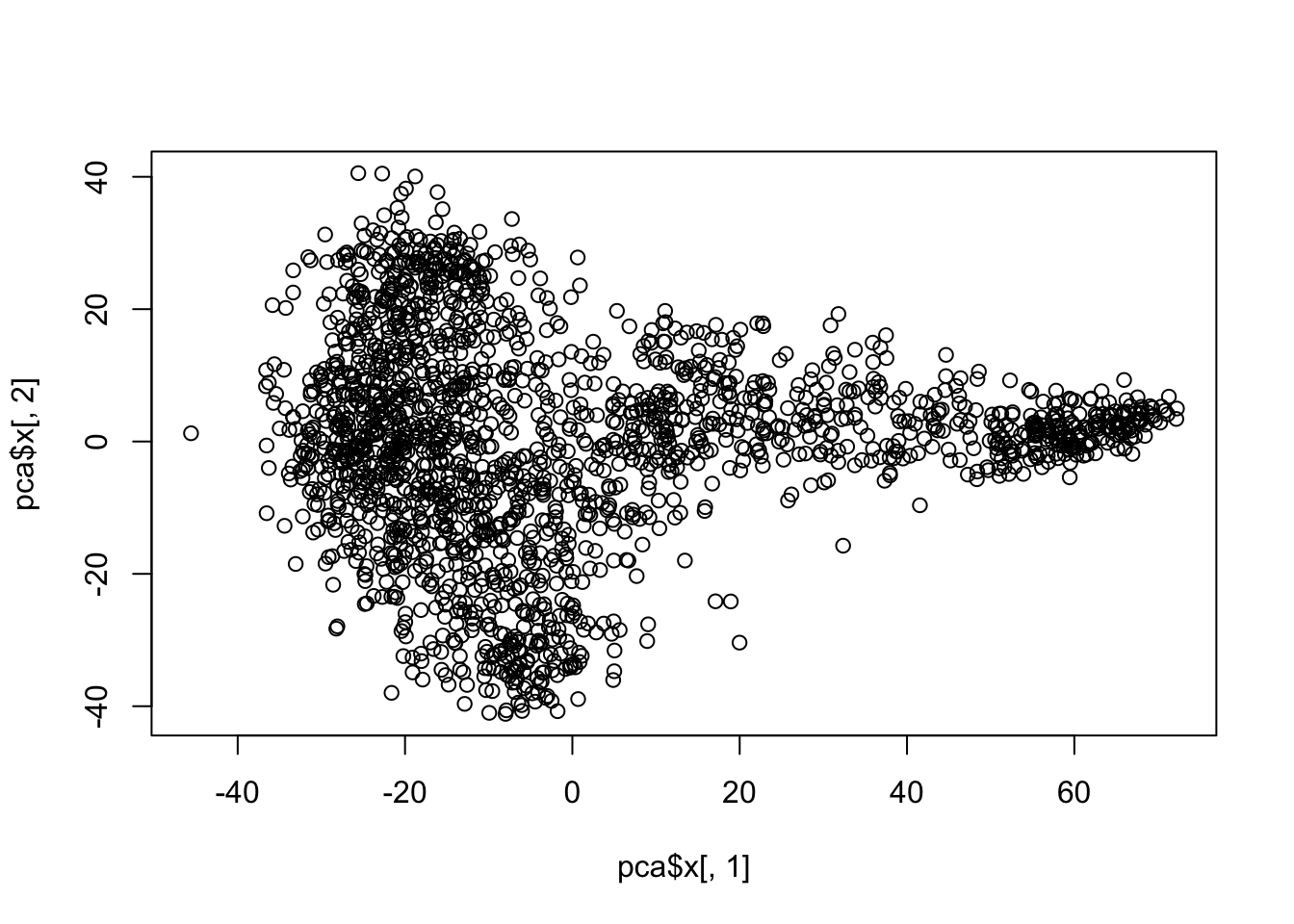
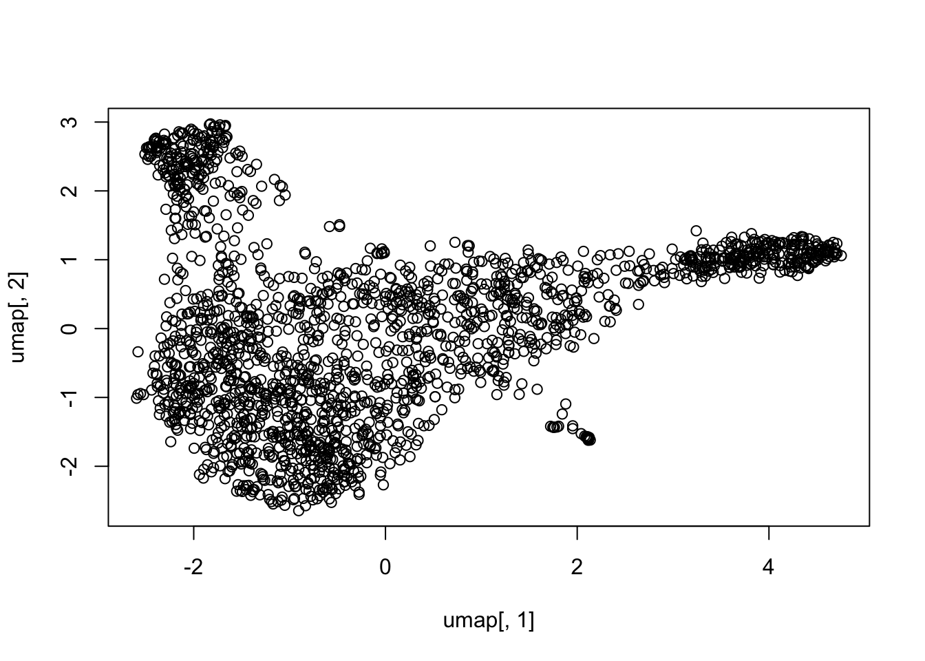
ENSMUSG00000026358 . 8.2269 8.2393 9.3669 1.89216 4.2094 4.3091 10.68693 8.4872 . We will see more advanced ways of reducing scRNAseq data dimensionality in the coming lectures and labs.
Seurat is another very popular ecosystem to investigate scRNAseq data. It is primarily developed and maintained by the Sajita Lab. It originally begun as a single package aiming at encompassing “all” (most) aspects of scRNAseq analysis. However, it rapidly evolved in a much larger project, and now operates along with other “wrappers” and extensions. It also has a very extended support from the lab group. All in all, is provides a (somewhat) simple workflow to start investigating scRNAseq data.
It is important to chose one standard that you feel comfortable with yourself. Which standard provides the most intuitive approach for you? Do you prefer an “all-in-one, plug-n-play” workflow (Seurat-style), or a modular approach (Bioconductor-style)? Which documentation is easier to read for you, a central full-featured website with extensive examples (Seurat-style), or “programmatic”-style vignettes (Bioconductor-style)?
This course will mostly rely on Bioconductor-based methods, but sometimes use Seurat-based methods.s In the absence of coordination of data structures, the next best solution is to write functions to coerce an object from a certain class to another class (i.e. Seurat to SingleCellExperiment, or vice-versa). Luckily, this is quite straightforward in R for these 2 data classes:
R
sce_seurat <- Seurat::as.Seurat(sce)Warning: Keys should be one or more alphanumeric characters followed by an underscore, setting key from DC to DC_sceclass: SingleCellExperiment
dim: 500 1920
metadata(0):
assays(2): counts logcounts
rownames(500): ENSMUSG00000076609 ENSMUSG00000021250 ... ENSMUSG00000026000 ENSMUSG00000005982
rowData names(0):
colnames(1920): HSPC_007 HSPC_013 ... Prog_852 Prog_810
colData names(11): gate broad ... label sizeFactor
reducedDimNames(1): diffusion
mainExpName: endogenous
altExpNames(0):sce_seuratAn object of class Seurat
500 features across 1920 samples within 1 assay
Active assay: endogenous (500 features, 0 variable features)
2 layers present: counts, data
1 dimensional reduction calculated: diffusionsce2 <- Seurat::as.SingleCellExperiment(sce_seurat)Public single-cell RNA-seq data can be retrieved from within R directly, thanks to several data packages, for instance scRNAseq or HCAData.
The interest of this approach is that one can recover a full-fledged SingleCellExperiment (often) provided by the authors of the corresponding study. This means that lots of information, such as batch ID, clustering, cell annotation, etc., may be readily available.
To compare the two different approaches, try preparing both a SingleCellExperiment or a Seurat object from scratch, using the matrix files generated in the previous lab. Read the documentation of the two related packages to understand how to do this.
This will be extensively covered in the next lab for everybody.