9  Lab 5: Dimension reduction, clustering and annotation

Notes

The estimated time for this lab is around 1h20.

Aims

• Learn how to perform dimension reduction on scRNAseq data
• Understand the importance of feature selection
• Learn how to perform clustering on scRNAseq data
• Learn how to (automatically) annotate cells based on clustering results

9.1 Dimensional reduction for clustering

9.1.1 Preparing dataset

We will prepare scRNAseq data from a PBMC run, provided by 10X and hosted by Bioconductor as a package.

Question

Which package from Bioconductor gives streamlined access to PBMC scRNAseq dataset from 10X Genomics?

What does the object contain (type of data, number of cells, batches, organism, …)? Can you get the same data from somewhere else?

Answer

R

library(tidyverse)

── Attaching core tidyverse packages ──────────────────────────────────────────────────────────────────────────────────────────────────────────────────────────────────────────────── tidyverse 2.0.0 ──
✔ dplyr     1.1.4     ✔ readr     2.1.5
✔ forcats   1.0.0     ✔ stringr   1.5.1
✔ ggplot2   3.5.1     ✔ tibble    3.2.1
✔ lubridate 1.9.3     ✔ tidyr     1.3.1
✔ purrr     1.0.2     
── Conflicts ────────────────────────────────────────────────────────────────────────────────────────────────────────────────────────────────────────────────────────────────── tidyverse_conflicts() ──
✖ dplyr::filter() masks stats::filter()
✖ dplyr::lag()    masks stats::lag()
ℹ Use the conflicted package (<http://conflicted.r-lib.org/>) to force all conflicts to become errors

library(SingleCellExperiment)

Loading required package: SummarizedExperiment
Loading required package: MatrixGenerics
Loading required package: matrixStats

Attaching package: 'matrixStats'

The following object is masked from 'package:dplyr':

    count


Attaching package: 'MatrixGenerics'

The following objects are masked from 'package:matrixStats':

    colAlls, colAnyNAs, colAnys, colAvgsPerRowSet, colCollapse, colCounts, colCummaxs, colCummins, colCumprods, colCumsums, colDiffs, colIQRDiffs, colIQRs, colLogSumExps,
    colMadDiffs, colMads, colMaxs, colMeans2, colMedians, colMins, colOrderStats, colProds, colQuantiles, colRanges, colRanks, colSdDiffs, colSds, colSums2, colTabulates,
    colVarDiffs, colVars, colWeightedMads, colWeightedMeans, colWeightedMedians, colWeightedSds, colWeightedVars, rowAlls, rowAnyNAs, rowAnys, rowAvgsPerColSet, rowCollapse,
    rowCounts, rowCummaxs, rowCummins, rowCumprods, rowCumsums, rowDiffs, rowIQRDiffs, rowIQRs, rowLogSumExps, rowMadDiffs, rowMads, rowMaxs, rowMeans2, rowMedians, rowMins,
    rowOrderStats, rowProds, rowQuantiles, rowRanges, rowRanks, rowSdDiffs, rowSds, rowSums2, rowTabulates, rowVarDiffs, rowVars, rowWeightedMads, rowWeightedMeans,
    rowWeightedMedians, rowWeightedSds, rowWeightedVars

Loading required package: GenomicRanges
Loading required package: stats4
Loading required package: BiocGenerics

Attaching package: 'BiocGenerics'

The following objects are masked from 'package:lubridate':

    intersect, setdiff, union

The following objects are masked from 'package:dplyr':

    combine, intersect, setdiff, union

The following objects are masked from 'package:stats':

    IQR, mad, sd, var, xtabs

The following objects are masked from 'package:base':

    anyDuplicated, aperm, append, as.data.frame, basename, cbind, colnames, dirname, do.call, duplicated, eval, evalq, Filter, Find, get, grep, grepl, intersect, is.unsorted,
    lapply, Map, mapply, match, mget, order, paste, pmax, pmax.int, pmin, pmin.int, Position, rank, rbind, Reduce, rownames, sapply, setdiff, table, tapply, union, unique,
    unsplit, which.max, which.min

Loading required package: S4Vectors

Attaching package: 'S4Vectors'

The following objects are masked from 'package:lubridate':

    second, second<-

The following objects are masked from 'package:dplyr':

    first, rename

The following object is masked from 'package:tidyr':

    expand

The following object is masked from 'package:utils':

    findMatches

The following objects are masked from 'package:base':

    expand.grid, I, unname

Loading required package: IRanges

Attaching package: 'IRanges'

The following object is masked from 'package:lubridate':

    %within%

The following objects are masked from 'package:dplyr':

    collapse, desc, slice

The following object is masked from 'package:purrr':

    reduce

Loading required package: GenomeInfoDb
Loading required package: Biobase
Welcome to Bioconductor

    Vignettes contain introductory material; view with 'browseVignettes()'. To cite Bioconductor, see 'citation("Biobase")', and for packages 'citation("pkgname")'.


Attaching package: 'Biobase'

The following object is masked from 'package:MatrixGenerics':

    rowMedians

The following objects are masked from 'package:matrixStats':

    anyMissing, rowMedians

sce <- TENxPBMCData::TENxPBMCData('pbmc4k')

see ?TENxPBMCData and browseVignettes('TENxPBMCData') for documentation
loading from cache

rownames(sce) <- scuttle::uniquifyFeatureNames(rowData(sce)$ENSEMBL_ID, rowData(sce)$Symbol_TENx)
sce

class: SingleCellExperiment 
dim: 33694 4340 
metadata(0):
assays(1): counts
rownames(33694): RP11-34P13.3 FAM138A ... AC213203.1 FAM231B
rowData names(3): ENSEMBL_ID Symbol_TENx Symbol
colnames: NULL
colData names(11): Sample Barcode ... Individual Date_published
reducedDimNames(0):
mainExpName: NULL
altExpNames(0):

rowData(sce)

DataFrame with 33694 rows and 3 columns
                  ENSEMBL_ID  Symbol_TENx       Symbol
                 <character>  <character>  <character>
RP11-34P13.3 ENSG00000243485 RP11-34P13.3           NA
FAM138A      ENSG00000237613      FAM138A      FAM138A
OR4F5        ENSG00000186092        OR4F5        OR4F5
RP11-34P13.7 ENSG00000238009 RP11-34P13.7 LOC100996442
RP11-34P13.8 ENSG00000239945 RP11-34P13.8           NA
...                      ...          ...          ...
AC233755.2   ENSG00000277856   AC233755.2           NA
AC233755.1   ENSG00000275063   AC233755.1 LOC102723407
AC240274.1   ENSG00000271254   AC240274.1 LOC102724250
AC213203.1   ENSG00000277475   AC213203.1           NA
FAM231B      ENSG00000268674      FAM231B      FAM231C

colData(sce)

DataFrame with 4340 rows and 11 columns
          Sample            Barcode         Sequence   Library Cell_ranger_version Tissue_status Barcode_type   Chemistry Sequence_platform    Individual Date_published
     <character>        <character>      <character> <integer>         <character>   <character>  <character> <character>       <character>   <character>    <character>
1         pbmc4k AAACCTGAGAAGGCCT-1 AAACCTGAGAAGGCCT         1                v2.1            NA     Chromium Chromium_v2         Hiseq4000 HealthyDonor1     2017-11-08
2         pbmc4k AAACCTGAGACAGACC-1 AAACCTGAGACAGACC         1                v2.1            NA     Chromium Chromium_v2         Hiseq4000 HealthyDonor1     2017-11-08
3         pbmc4k AAACCTGAGATAGTCA-1 AAACCTGAGATAGTCA         1                v2.1            NA     Chromium Chromium_v2         Hiseq4000 HealthyDonor1     2017-11-08
4         pbmc4k AAACCTGAGCGCCTCA-1 AAACCTGAGCGCCTCA         1                v2.1            NA     Chromium Chromium_v2         Hiseq4000 HealthyDonor1     2017-11-08
5         pbmc4k AAACCTGAGGCATGGT-1 AAACCTGAGGCATGGT         1                v2.1            NA     Chromium Chromium_v2         Hiseq4000 HealthyDonor1     2017-11-08
...          ...                ...              ...       ...                 ...           ...          ...         ...               ...           ...            ...
4336      pbmc4k TTTGGTTTCGCTAGCG-1 TTTGGTTTCGCTAGCG         1                v2.1            NA     Chromium Chromium_v2         Hiseq4000 HealthyDonor1     2017-11-08
4337      pbmc4k TTTGTCACACTTAACG-1 TTTGTCACACTTAACG         1                v2.1            NA     Chromium Chromium_v2         Hiseq4000 HealthyDonor1     2017-11-08
4338      pbmc4k TTTGTCACAGGTCCAC-1 TTTGTCACAGGTCCAC         1                v2.1            NA     Chromium Chromium_v2         Hiseq4000 HealthyDonor1     2017-11-08
4339      pbmc4k TTTGTCAGTTAAGACA-1 TTTGTCAGTTAAGACA         1                v2.1            NA     Chromium Chromium_v2         Hiseq4000 HealthyDonor1     2017-11-08
4340      pbmc4k TTTGTCATCCCAAGAT-1 TTTGTCATCCCAAGAT         1                v2.1            NA     Chromium Chromium_v2         Hiseq4000 HealthyDonor1     2017-11-08

table(sce$Library)

   1 
4340 

9.1.2 Normalize counts using scran

Just like in bulk high-throughput sequencing experiments, scRNAseq counts have to be normalized to the sequencing depth for each cell. We can define the library size as the total sum of counts across all genes for each cell, the expected value of which is assumed to scale with any cell-specific biases. However, this relies on the assumption that within the entire dataset, most genes are non-differentially expressed and expressed roughly within the same range. Depending on the set up of the scRNAseq experiment, this can be entirely false. To avoid relying on this hypothesis, we can (1) quickly pre-cluster cells, then (2) normalize cells using their library size factor separately in each cluster, then (3) rescaling size factors so that they are comparable across clusters.

All of this can be done very simply using the combo quickCluster() + computeSumFactors() + logNormCounts() from scran/scuttle packages.

Question

What is the purpose of the quickCluster() function? What does it return?

What is the purpose of the computeSumFactors() function? What does it return?

What is the purpose of the logNormCounts() function? What does it return?

Answer

R

clusters <- scran::quickCluster(sce)
table(clusters)

clusters
  1   2   3   4   5   6   7   8   9  10  11 
588 361 264 161 866 365 531 536 360 207 101 

sce <- scran::computeSumFactors(sce, cluster = clusters)
colData(sce)

DataFrame with 4340 rows and 12 columns
          Sample            Barcode         Sequence   Library Cell_ranger_version Tissue_status Barcode_type   Chemistry Sequence_platform    Individual Date_published sizeFactor
     <character>        <character>      <character> <integer>         <character>   <character>  <character> <character>       <character>   <character>    <character>  <numeric>
1         pbmc4k AAACCTGAGAAGGCCT-1 AAACCTGAGAAGGCCT         1                v2.1            NA     Chromium Chromium_v2         Hiseq4000 HealthyDonor1     2017-11-08   0.403246
2         pbmc4k AAACCTGAGACAGACC-1 AAACCTGAGACAGACC         1                v2.1            NA     Chromium Chromium_v2         Hiseq4000 HealthyDonor1     2017-11-08   0.739777
3         pbmc4k AAACCTGAGATAGTCA-1 AAACCTGAGATAGTCA         1                v2.1            NA     Chromium Chromium_v2         Hiseq4000 HealthyDonor1     2017-11-08   0.429493
4         pbmc4k AAACCTGAGCGCCTCA-1 AAACCTGAGCGCCTCA         1                v2.1            NA     Chromium Chromium_v2         Hiseq4000 HealthyDonor1     2017-11-08   0.527001
5         pbmc4k AAACCTGAGGCATGGT-1 AAACCTGAGGCATGGT         1                v2.1            NA     Chromium Chromium_v2         Hiseq4000 HealthyDonor1     2017-11-08   0.600344
...          ...                ...              ...       ...                 ...           ...          ...         ...               ...           ...            ...        ...
4336      pbmc4k TTTGGTTTCGCTAGCG-1 TTTGGTTTCGCTAGCG         1                v2.1            NA     Chromium Chromium_v2         Hiseq4000 HealthyDonor1     2017-11-08   1.422566
4337      pbmc4k TTTGTCACACTTAACG-1 TTTGTCACACTTAACG         1                v2.1            NA     Chromium Chromium_v2         Hiseq4000 HealthyDonor1     2017-11-08   0.947146
4338      pbmc4k TTTGTCACAGGTCCAC-1 TTTGTCACAGGTCCAC         1                v2.1            NA     Chromium Chromium_v2         Hiseq4000 HealthyDonor1     2017-11-08   1.962193
4339      pbmc4k TTTGTCAGTTAAGACA-1 TTTGTCAGTTAAGACA         1                v2.1            NA     Chromium Chromium_v2         Hiseq4000 HealthyDonor1     2017-11-08   0.615199
4340      pbmc4k TTTGTCATCCCAAGAT-1 TTTGTCATCCCAAGAT         1                v2.1            NA     Chromium Chromium_v2         Hiseq4000 HealthyDonor1     2017-11-08   0.771550

sce <- scuttle::logNormCounts(sce)
assays(sce)

List of length 2
names(2): counts logcounts

9.1.3 Feature selection

We often use scRNAseq data in exploratory analyses to characterize heterogeneity across cells. Procedures like clustering and dimensionality reduction compare cells based on their gene expression profiles. The choice of genes to include in this comparison may have a major impact on the performance of downstream methods. Ideally, one wants to only select genes that contain useful information about the biology of the system while removing genes that contain random noise. This aims to preserve interesting biological structure without the variance that obscures that structure.

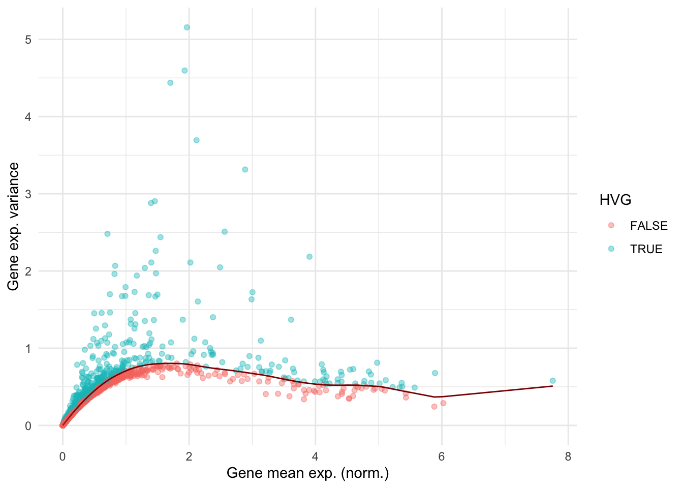
The simplest approach to feature selection is to compute the variance of the log-normalized expression values, to select the most variable genes. Modelling of the mean-variance relationship can be achieved by the modelGeneVar() function from the scran package.

Question

Apply the modelGeneVar() function to the normalized counts. What does the returned object contain?

Answer

R

sce_filtered_variance <- scran::modelGeneVar(sce)
sce_filtered_variance

DataFrame with 33694 rows and 6 columns
                    mean       total        tech          bio   p.value       FDR
               <numeric>   <numeric>   <numeric>    <numeric> <numeric> <numeric>
RP11-34P13.3 0.000000000 0.000000000 0.000000000  0.00000e+00       NaN       NaN
FAM138A      0.000000000 0.000000000 0.000000000  0.00000e+00       NaN       NaN
OR4F5        0.000000000 0.000000000 0.000000000  0.00000e+00       NaN       NaN
RP11-34P13.7 0.001973297 0.002003373 0.002046038 -4.26643e-05  0.549850  0.744658
RP11-34P13.8 0.000491705 0.000531807 0.000509831  2.19764e-05  0.397824  0.744658
...                  ...         ...         ...          ...       ...       ...
AC233755.2    0.00000000   0.0000000   0.0000000   0.00000000       NaN       NaN
AC233755.1    0.00000000   0.0000000   0.0000000   0.00000000       NaN       NaN
AC240274.1    0.00961767   0.0112683   0.0099722   0.00129611  0.217433  0.744658
AC213203.1    0.00000000   0.0000000   0.0000000   0.00000000       NaN       NaN
FAM231B       0.00000000   0.0000000   0.0000000   0.00000000       NaN       NaN

Identify the top 10% most variable genes from this object.

Answer

R

HVGs <- scran::getTopHVGs(sce_filtered_variance, prop = 0.1)
rowData(sce)$isHVG <- rownames(sce) %in% HVGs
head(rowData(sce))

DataFrame with 6 rows and 4 columns
                   ENSEMBL_ID   Symbol_TENx       Symbol     isHVG
                  <character>   <character>  <character> <logical>
RP11-34P13.3  ENSG00000243485  RP11-34P13.3           NA     FALSE
FAM138A       ENSG00000237613       FAM138A      FAM138A     FALSE
OR4F5         ENSG00000186092         OR4F5        OR4F5     FALSE
RP11-34P13.7  ENSG00000238009  RP11-34P13.7 LOC100996442     FALSE
RP11-34P13.8  ENSG00000239945  RP11-34P13.8           NA     FALSE
RP11-34P13.14 ENSG00000239906 RP11-34P13.14           NA     FALSE

table(rowData(sce)$isHVG)

FALSE  TRUE 
32424  1270 

Visualize the mean-variance fit of the data, coloring points by whether they are in the top 10% most variable genes.

Answer

R

df <- tibble(
    mean = metadata(sce_filtered_variance)$mean, 
    var = metadata(sce_filtered_variance)$var, 
    trend = metadata(sce_filtered_variance)$trend(mean), 
    HVG = rowData(sce)$isHVG
)
ggplot(df) + 
    geom_point(aes(x = mean, y = var, col = HVG), alpha = 0.4) + 
    geom_line(aes(x = mean, y = trend), col = 'darkred') +
    theme_minimal() + 
    labs(x = 'Gene mean exp. (norm.)', y = 'Gene exp. variance')

9.1.4 PCA on filtered dataset

We now have normalized counts filtered for the top 500 genes varying with the greatest biological significance.
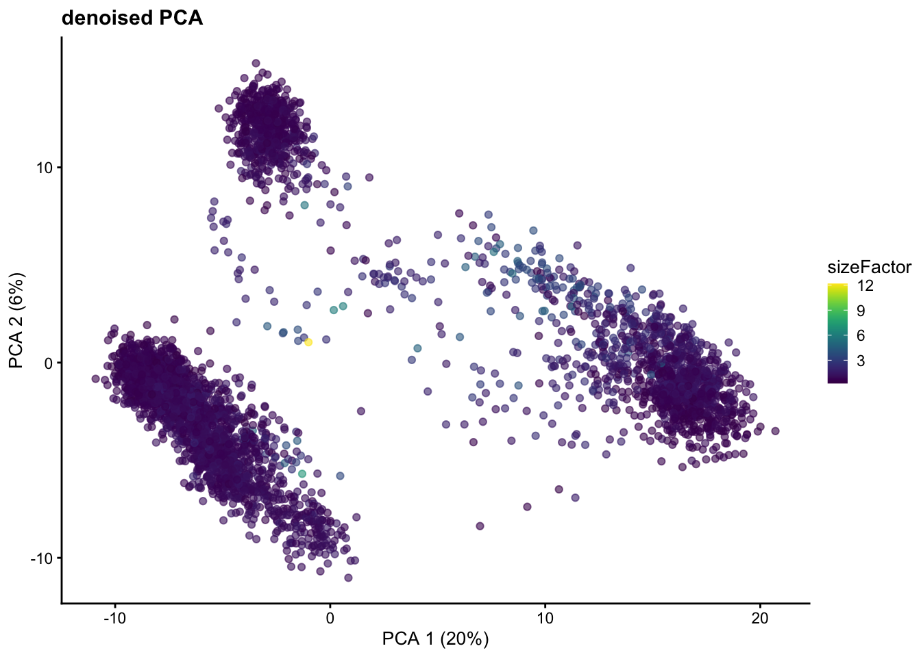
Still, that represents a 500 x nCells (~8,000) dataset (each row being a feature). This is still too big to reliably use in standard clustering approaches. We can further compress the dataset. The most widely used approach is PCA: it computes a small number of “components” (typically 5-50) optimally summarizing the variability of the whole dataset, while retaining linearity of the underlying numerical data and being computationallt quite efficient.

Question

Leverage the scater package to compute a PCA embedding of the filtered data by taking into account the technical variability.

Answer

R

sce <- scran::denoisePCA(
    sce, 
    technical = sce_filtered_variance, 
    subset.row = HVGs, 
    min.rank = 15
)
p <- scater::plotReducedDim(sce, 'PCA', colour_by = 'sizeFactor') + ggtitle('denoised PCA')
p

9.2 Clustering

Clustering is an unsupervised learning procedure that is used in scRNA-seq data analysis to empirically define groups of cells with similar expression profiles. Its primary purpose is to summarize the data in a digestible format for human interpretation.

After annotation based on marker genes, the clusters can be treated as proxies for more abstract biological concepts such as cell types or states. Clustering is thus a critical step for extracting biological insights from scRNA-seq data.

9.2.1 Clustering algorithms

Three main approaches can be used:

1. Hierarchical clustering
2. k-means clustering
3. Graph-based clustering

Today, we will focus on graph-based clustering, as it is becoming the standard for scRNAseq: it is a flexible and scalable technique for clustering even the largest scRNA-seq datasets. We first build a graph where each node is a cell that is connected by edges to its nearest neighbors in the high-dimensional space. Edges are weighted based on the similarity between the cells involved, with higher weight given to cells that are more closely related.

Question

Compute a graph-based clustering of the PBMC dataset.

Answer

R

graph <- scran::buildSNNGraph(
    sce, 
    k = 5, 
    use.dimred = 'PCA'
)
sce_clust <- igraph::cluster_louvain(graph)$membership
sce$clusters_graph <- factor(sce_clust)
table(sce$clusters_graph)

  1   2   3   4   5   6   7   8   9  10  11  12  13  14  15  16  17 
502 359 682  40 129 393  61 193 349 363 376 218 190 151 127 197  10 

Question

What are the main parameters to choose when building the graph? How do they impact the clustering?

Answer

R

graph2 <- scran::buildSNNGraph(
    sce, 
    k = 50, 
    use.dimred = 'PCA'
)
sce_clust2 <- igraph::cluster_louvain(graph2)$membership
table(sce_clust, sce_clust2)

         sce_clust2
sce_clust   1   2   3   4   5   6   7   8
       1  502   0   0   0   0   0   0   0
       2    0 321  29   0   0   9   0   0
       3    0  23 659   0   0   0   0   0
       4    0   0   0  37   1   0   2   0
       5   23   0   0 106   0   0   0   0
       6    0   1   0   0 389   3   0   0
       7   58   0   1   0   2   0   0   0
       8    0 181  12   0   0   0   0   0
       9    0   1 348   0   0   0   0   0
       10 363   0   0   0   0   0   0   0
       11   0   1   0   0   0 374   1   0
       12   0   0   0   0 218   0   0   0
       13   0   0   0   0   1  22 167   0
       14   0   0   0   0   0 151   0   0
       15  14   0   0   1   0   0   0 112
       16   0 167   1   0   0  29   0   0
       17   0   5   2   0   3   0   0   0

9.2.2 Dimensional reduction for clustering visualization

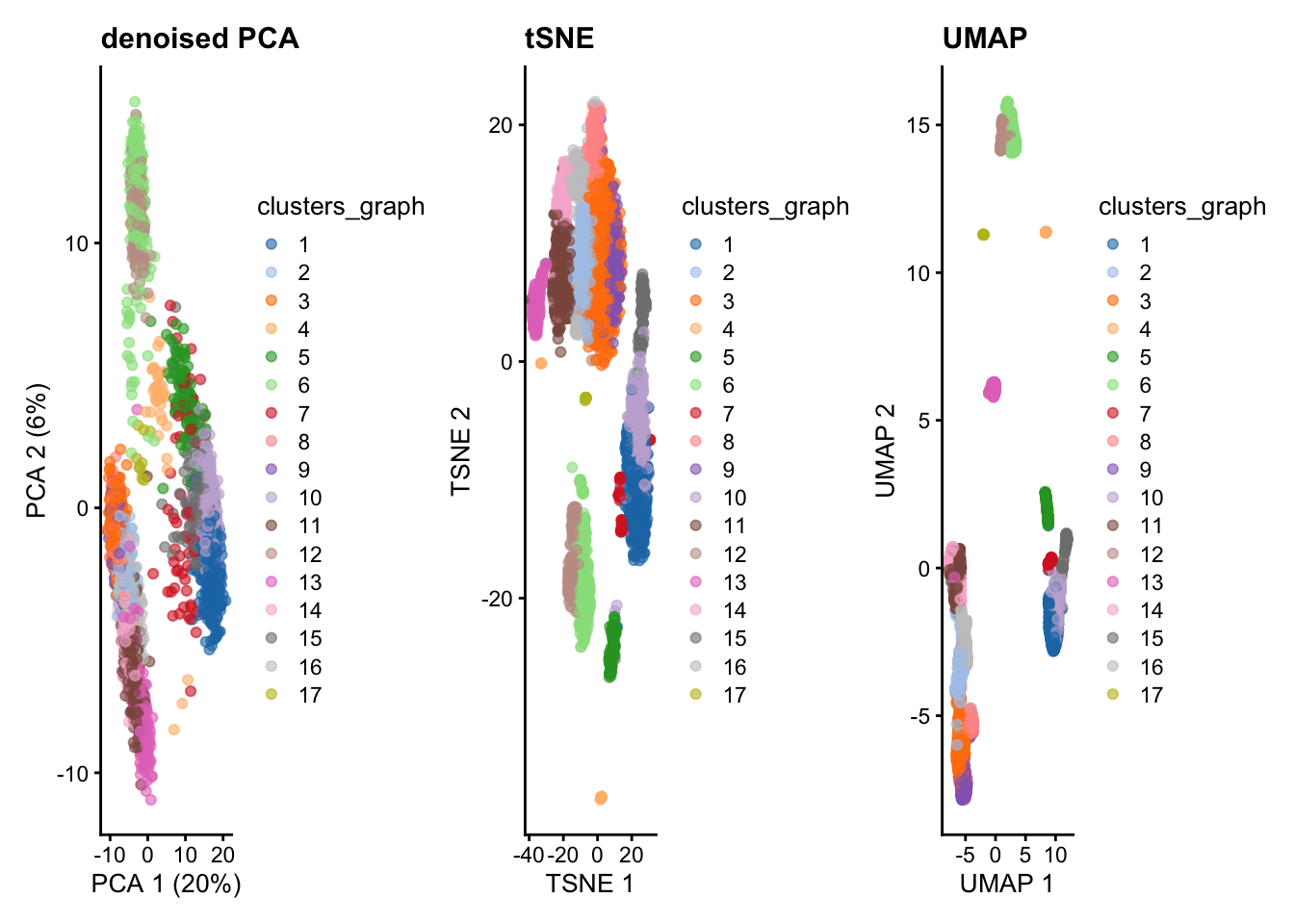
PCA is a powerful linear approach to compress large datasets into smaller dimensional spaces. However, it struggles at emphasizing the existence of clusters in complex datasets, when visualized in 2D.

scater provides a handy way to perform more complex data embeddings:

- tSNE
- UMAP
- Diffusion Map
- Multi-Dimensional Scaling (MDS)
- Non-negative Matrix Factorization (NMF)

Question

Explore the different dimensional reduction algorithms, trying different hyperparameters combinations.

When you run these commands, pay attention to how long each command takes to run! While this run, check the Help page for each function (e.g. ?runTSNE)

Answer

R

reducedDims(sce)

List of length 1
names(1): PCA

sce <- scater::runTSNE(sce, subset_row = HVGs)
sce <- scater::runUMAP(sce, subset_row = HVGs)
reducedDims(sce)

List of length 3
names(3): PCA TSNE UMAP

reducedDim(sce, 'UMAP')[1:10, ]

        UMAP1    UMAP2
 [1,] 10.4762 -1.74452
 [2,]  9.9714 -1.70896
 [3,]  8.9500 -1.36885
 [4,] -6.3458 -3.38246
 [5,] -5.7974 -6.26426
 [6,] -6.6016 -1.30995
 [7,]  8.3734 11.37350
 [8,]  8.4162  2.35892
 [9,]  2.7606 14.29711
[10,]  8.8376  0.10778

Question

Use the scater::plotReducedDim() function to plot cells in each embedding. Comment.

Answer

R

library(patchwork)
p<- scater::plotReducedDim(sce, 'PCA', colour_by = 'clusters_graph') + ggtitle('denoised PCA') +
    scater::plotReducedDim(sce, 'TSNE', colour_by = 'clusters_graph') + ggtitle('tSNE') +
    scater::plotReducedDim(sce, 'UMAP', colour_by = 'clusters_graph') + ggtitle('UMAP')
p

9.2.3 BONUS For the pros of clustering… Compare different clustering approaches

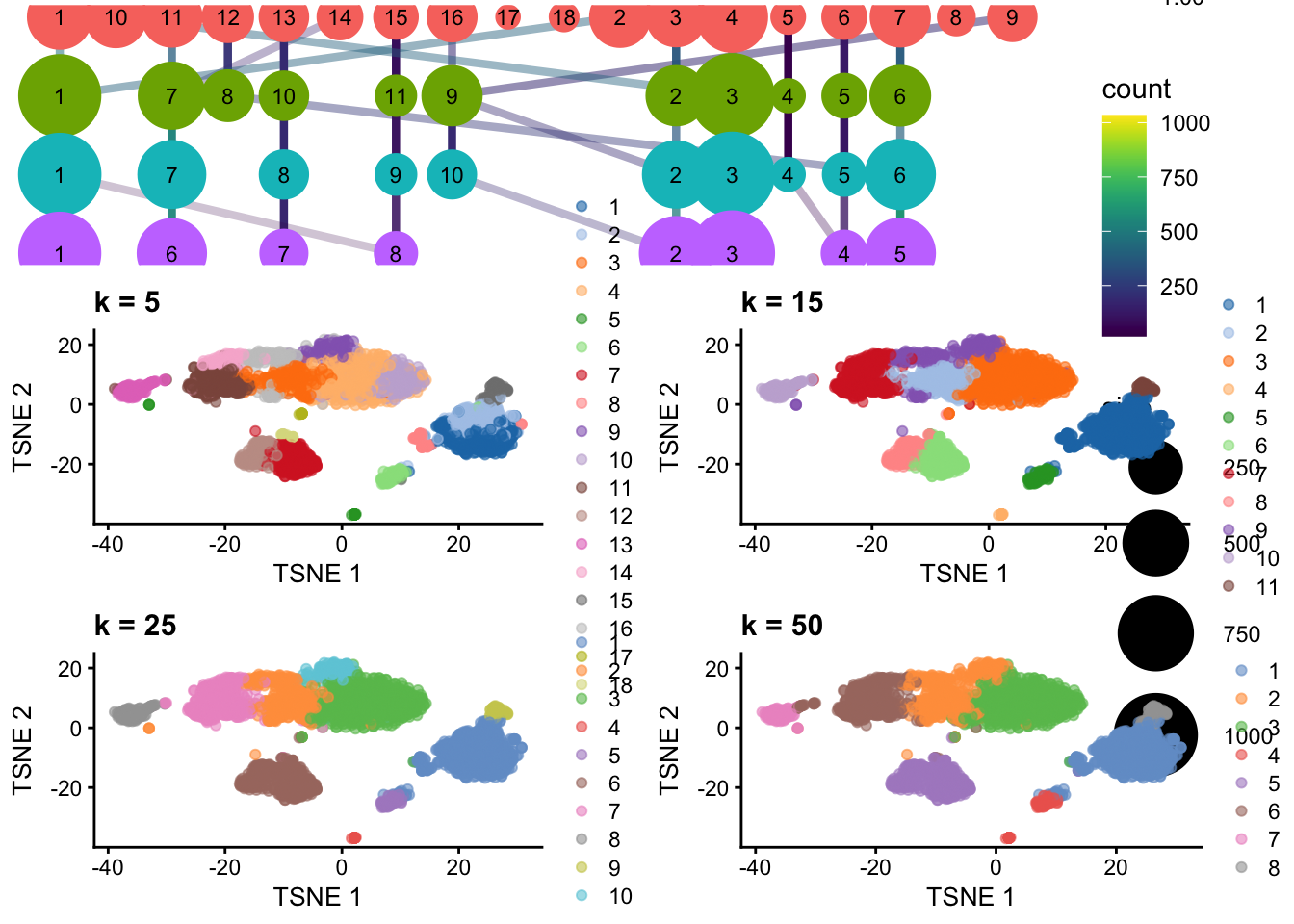
Leveraging the bluster package, different clustering approaches can be performed using a uniformed syntax, to compare their output.

Question

Using clusterSweep(), compare the effect of different k neighbor values when performing graph-based clustering.

Answer

R

clusters <- bluster::clusterSweep(
    reducedDim(sce, 'PCA'), 
    BLUSPARAM = bluster::SNNGraphParam(),
    k = c(5L, 15L, 25L, 50L), 
    cluster.fun = c("louvain")
)
colnames(clusters$clusters)

[1] "k.5_cluster.fun.louvain"  "k.15_cluster.fun.louvain" "k.25_cluster.fun.louvain" "k.50_cluster.fun.louvain"

head(clusters$clusters)

DataFrame with 6 rows and 4 columns
  k.5_cluster.fun.louvain k.15_cluster.fun.louvain k.25_cluster.fun.louvain k.50_cluster.fun.louvain
                 <factor>                 <factor>                 <factor>                 <factor>
1                       1                        1                        1                        1
2                       2                        1                        1                        1
3                       1                        1                        1                        1
4                       3                        2                        2                        2
5                       4                        3                        3                        3
6                       3                        2                        3                        3

clusters$parameters

DataFrame with 4 rows and 2 columns
                                 k cluster.fun
                         <integer> <character>
k.5_cluster.fun.louvain          5     louvain
k.15_cluster.fun.louvain        15     louvain
k.25_cluster.fun.louvain        25     louvain
k.50_cluster.fun.louvain        50     louvain

library(ggraph)
p <- cowplot::plot_grid(
    clustree::clustree(
        clusters$clusters %>% setNames(1:ncol(.)) %>% as.data.frame(),
        prefix = 'X',
        edge_arrow=FALSE
    ), 
    cowplot::plot_grid(
        scater::plotReducedDim(sce, 'TSNE', colour_by = I(clusters$clusters[, 'k.5_cluster.fun.louvain'])) + ggtitle('k = 5'),
        scater::plotReducedDim(sce, 'TSNE', colour_by = I(clusters$clusters[, 'k.15_cluster.fun.louvain'])) + ggtitle('k = 15'),
        scater::plotReducedDim(sce, 'TSNE', colour_by = I(clusters$clusters[, 'k.25_cluster.fun.louvain'])) + ggtitle('k = 25'),
        scater::plotReducedDim(sce, 'TSNE', colour_by = I(clusters$clusters[, 'k.50_cluster.fun.louvain'])) + ggtitle('k = 50')
    ), 
    nrow = 2, 
    rel_heights = c(0.3, 0.7)
)
p

table(clusters$clusters[, 'k.5_cluster.fun.louvain'])

  1   2   3   4   5   6   7   8   9  10  11  12  13  14  15  16  17  18 
473 393 368 627  40 129 376  61 188 404 382 217 190 141 126 197  10  18 

9.3 Cell annotation

9.3.1 Find marker genes

To interpret clustering results, one needs to identify the genes that drive separation between clusters. These marker genes allow to assign biological meaning to each cluster based on their functional annotation. In the most obvious case, the marker genes for each cluster are a priori associated with particular cell types, allowing us to treat the clustering as a proxy for cell type identity.

A general strategy is to perform DE tests between pairs of clusters and then combine results into a single ranking of marker genes for each cluster.

R

markers <- scran::findMarkers(sce, groups = sce$clusters_graph)

Question

Find markers strongly overexpressed in each cluster. Check ?scran::findMarkers to find the right options to use.

Answer

R

markers <- scran::findMarkers(
    sce, 
    groups = sce$clusters_graph, 
    direction = "up", 
    lfc = 1
)
head(markers[[1]])

DataFrame with 6 rows and 20 columns
                    Top      p.value          FDR summary.logFC   logFC.2   logFC.3   logFC.4   logFC.5   logFC.6   logFC.7   logFC.8   logFC.9  logFC.10  logFC.11  logFC.12  logFC.13  logFC.14
              <integer>    <numeric>    <numeric>     <numeric> <numeric> <numeric> <numeric> <numeric> <numeric> <numeric> <numeric> <numeric> <numeric> <numeric> <numeric> <numeric> <numeric>
S100A9                1  0.00000e+00  0.00000e+00       5.41682   5.43237   5.41682   5.38506  3.527516   5.40582  1.300493   5.30313   5.29337  1.367411   5.51013   5.25562   5.57793   5.39685
S100A12               1 3.00254e-186 7.78211e-183       3.16760   3.14991   3.15614   3.06390  2.752834   3.16872  1.321253   3.13691   3.11275  1.428806   3.15624   3.14479   3.16760   3.13757
S100A8                1  0.00000e+00  0.00000e+00       5.35071   5.40804   5.35071   5.24867  4.002828   5.36811  1.429670   5.33249   5.42634  1.615361   5.44104   5.37566   5.57562   5.42914
MNDA                  1 6.44450e-174 1.35713e-170       2.69302   2.62331   2.65953   2.68560  1.039333   2.63823  0.869333   2.62066   2.66382  0.469773   2.68082   2.63842   2.69302   2.67460
LYZ                   1  0.00000e+00  0.00000e+00       5.27217   5.25980   5.27217   5.32183  0.755057   5.22486  0.992756   5.33170   5.26958  0.312196   5.30534   5.30214   5.49214   5.27623
RP11-1143G9.4         1 6.20347e-200 1.74183e-196       3.22726   3.16209   3.16589   3.04120  1.380130   3.16979  0.939639   3.18494   3.16750  0.865393   3.18003   3.17216   3.18095   3.22726
               logFC.15  logFC.16  logFC.17
              <numeric> <numeric> <numeric>
S100A9          4.11810   5.40420   5.33767
S100A12         3.05345   3.10968   3.06099
S100A8          4.62013   5.46970   5.41967
MNDA            1.17765   2.66604   2.70577
LYZ             3.03608   5.25555   5.19250
RP11-1143G9.4   2.72497   3.22522   3.21302

markers <- lapply(markers, function(df) {
    rownames(df[df$Top <= 5,])
})

Question

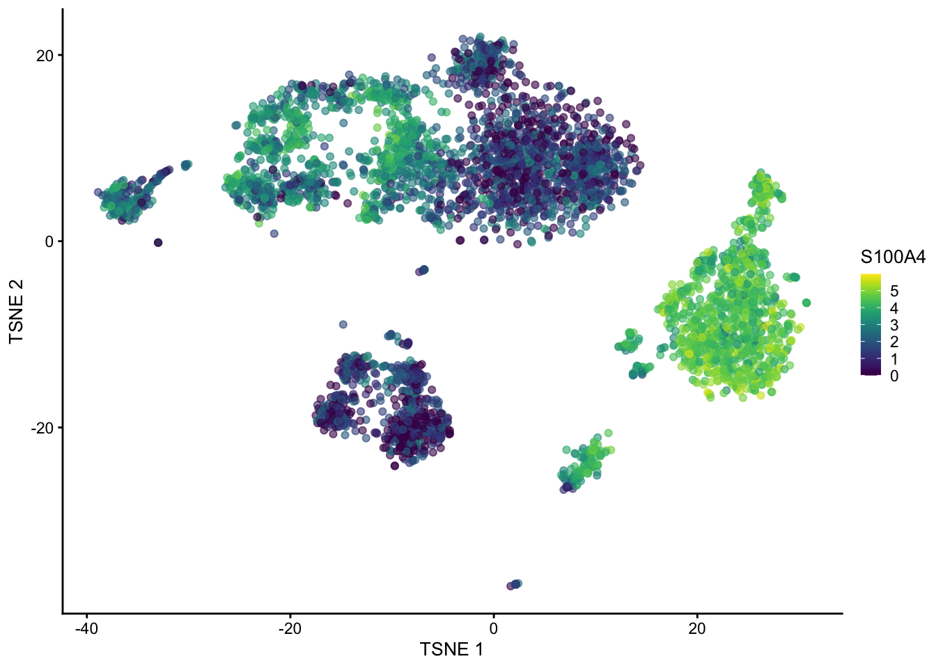
Plot average expression of the first marker of the first cluster in UMAP.

Answer

R

p <- scater::plotReducedDim(sce, 'TSNE', colour_by = markers[[2]][[1]])
p

9.3.2 Automated cell annotation

Many cell type reference databases are available over the Internet. Today, we will use a reference constructed from Blueprint and ENCODE data (Martens and Stunnenberg 2013; The ENCODE Project Consortium 2012). This reference is available as a SummarizedExperiment containing log-normalized gene expression for manually annotated samples.

R

ref <- celldex::BlueprintEncodeData()
prediction_types <- SingleR::SingleR(
    test = sce, 
    ref = ref, 
    labels = ref$label.main
)
sce$annotation <- prediction_types$labels
table(sce$annotation)

     B-cells CD4+ T-cells CD8+ T-cells           DC          HSC    Monocytes     NK cells 
         616          881         1390            1           14         1201          237 

table(sce$annotation, sce$clusters_graph)

              
                 1   2   3   4   5   6   7   8   9  10  11  12  13  14  15  16  17
  B-cells        0   0   0  14   0 383   0   0   0   0   0 218   0   0   0   0   1
  CD4+ T-cells   0 158 490   0   0   0   1  96  47   0   0   0   0   0   0  89   0
  CD8+ T-cells   0 201 192   0   0   9   0  97 302   0 342   0   3 136   0 108   0
  DC             0   0   0   0   1   0   0   0   0   0   0   0   0   0   0   0   0
  HSC            0   0   0   5   0   0   0   0   0   0   0   0   0   0   0   0   9
  Monocytes    502   0   0  21 128   0  60   0   0 363   0   0   0   0 127   0   0
  NK cells       0   0   0   0   0   1   0   0   0   0  34   0 187  15   0   0   0

Question

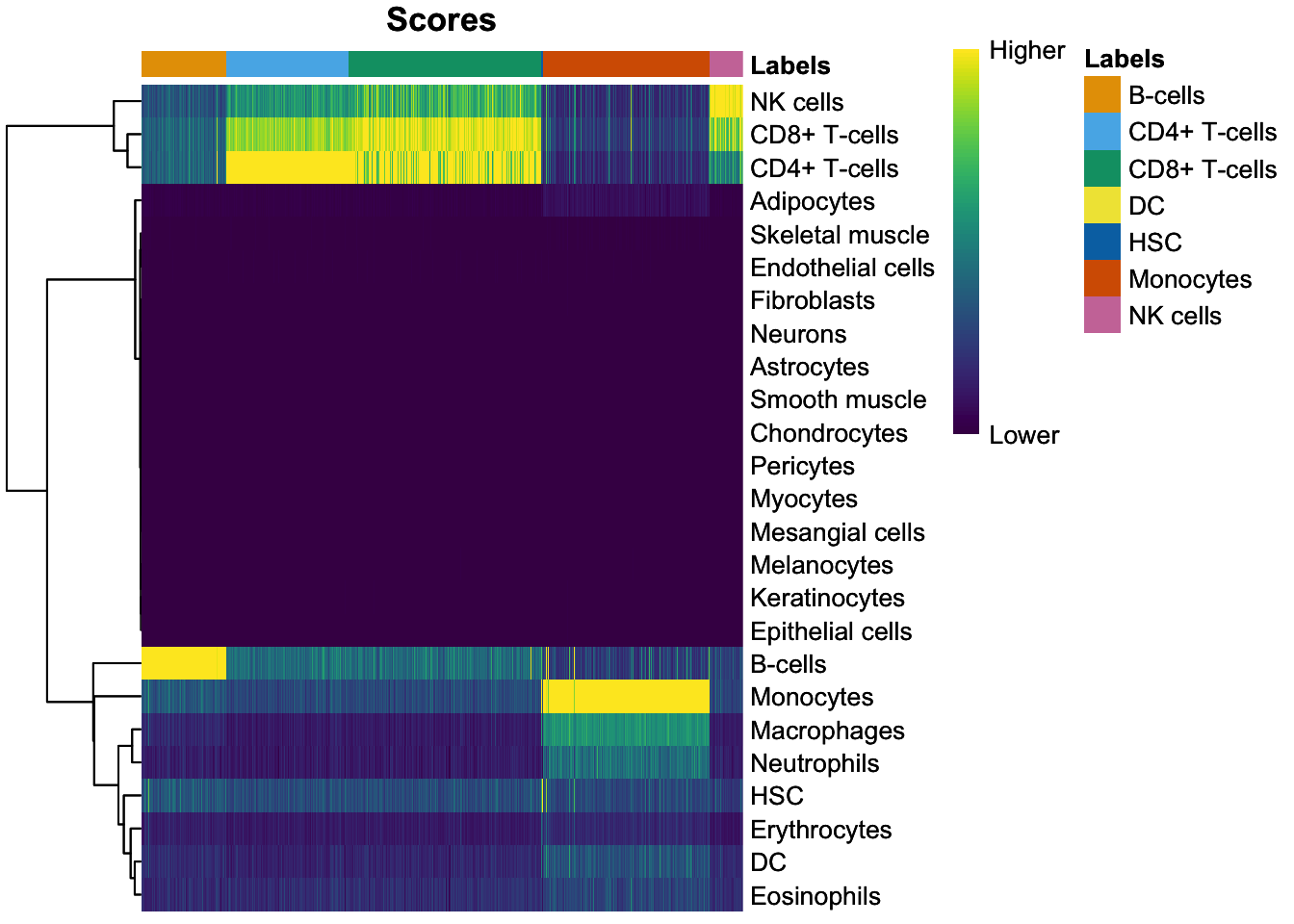
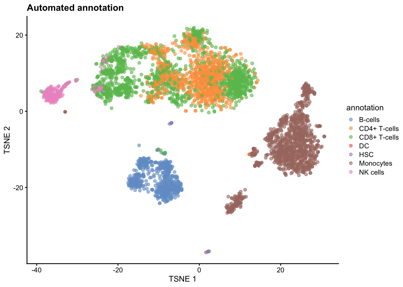
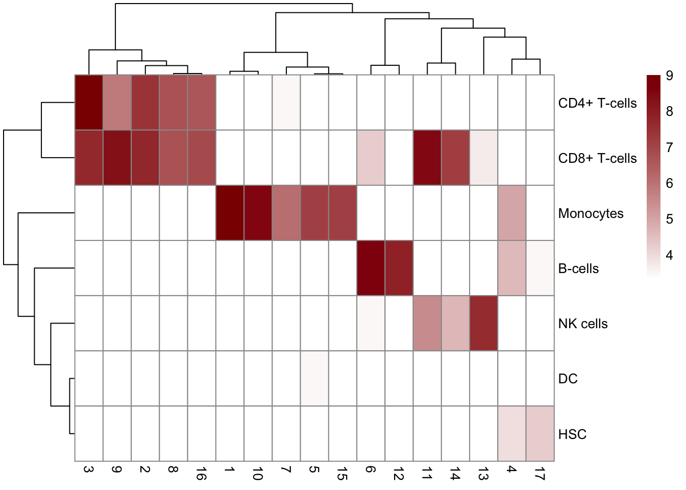
Using scater and SingleR utilities, visually compare the annotation scores for cells in each cluster.

Did the automated annotation work robuslty? How does it compare to our clustering? Is automated annotation as sensitive as graph-based clustering?

Answer

R

p <- SingleR::plotScoreHeatmap(prediction_types)
p

p <- scater::plotReducedDim(sce, 'TSNE', colour_by = 'annotation') + ggtitle('Automated annotation')
p

p <- pheatmap::pheatmap(
    log2(table(Annotation = sce$annotation, Cluster = sce$clusters_graph)+10), 
    color = colorRampPalette(c("white", "darkred"))(101)
)

9.4 Bonus

Try to fill in the analysis template in bin/prepare_Ernst.R to execute the different processing/analysis steps we covered in the previous exercises and this one. If you prefer using Seurat, don’t hesitate to modify the base template!

9.5 Acknowledgements

This exercise was adapted from Chapts. 7-12 of Orchestrating Single-Cell Analysis with Bioconductor.

9.6 Session info

─ Session info ───────────────────────────────────────────────────────────────────────────────────────────────────────────────────────────────────────────────────────────────────────────────────────
 setting  value
 version  R version 4.4.1 (2024-06-14)
 os       macOS Sonoma 14.6.1
 system   aarch64, darwin20
 ui       X11
 language (EN)
 collate  en_US.UTF-8
 ctype    en_US.UTF-8
 tz       Europe/Paris
 date     2024-11-03
 pandoc   2.19.2 @ /opt/homebrew/bin/ (via rmarkdown)

─ Packages ───────────────────────────────────────────────────────────────────────────────────────────────────────────────────────────────────────────────────────────────────────────────────────────
 package              * version  date (UTC) lib source
 abind                * 1.4-8    2024-09-12 [1] CRAN (R 4.4.1)
 alabaster.base         1.4.2    2024-06-23 [1] Bioconduc~
 alabaster.matrix       1.4.2    2024-06-23 [1] Bioconduc~
 alabaster.ranges       1.4.2    2024-06-23 [1] Bioconduc~
 alabaster.schemas      1.4.0    2024-04-30 [1] Bioconduc~
 alabaster.se           1.4.1    2024-05-30 [1] Bioconduc~
 AnnotationDbi          1.66.0   2024-06-16 [1] Bioconduc~
 AnnotationHub          3.12.0   2024-04-30 [1] Bioconduc~
 backports              1.5.0    2024-05-23 [1] CRAN (R 4.4.0)
 beachmat               2.20.0   2024-05-06 [1] Bioconduc~
 beeswarm               0.4.0    2021-06-01 [1] CRAN (R 4.4.0)
 Biobase              * 2.64.0   2024-04-30 [1] Bioconduc~
 BiocFileCache          2.12.0   2024-04-30 [1] Bioconduc~
 BiocGenerics         * 0.50.0   2024-04-30 [1] Bioconduc~
 BiocManager            1.30.25  2024-08-28 [1] CRAN (R 4.4.1)
 BiocNeighbors          1.22.0   2024-04-30 [1] Bioconduc~
 BiocParallel           1.38.0   2024-04-30 [1] Bioconduc~
 BiocSingular           1.20.0   2024-04-30 [1] Bioconduc~
 BiocVersion            3.19.1   2024-04-22 [1] Bioconduc~
 Biostrings             2.72.1   2024-06-02 [1] Bioconduc~
 bit                    4.5.0    2024-09-20 [1] CRAN (R 4.4.1)
 bit64                  4.5.2    2024-09-22 [1] CRAN (R 4.4.1)
 blob                   1.2.4    2023-03-17 [1] CRAN (R 4.4.0)
 bluster                1.14.0   2024-04-30 [1] Bioconduc~
 cachem                 1.1.0    2024-05-16 [1] CRAN (R 4.4.0)
 celldex                1.14.0   2024-05-02 [1] Bioconduc~
 checkmate              2.3.2    2024-07-29 [1] CRAN (R 4.4.0)
 cli                    3.6.3    2024-06-21 [1] CRAN (R 4.4.0)
 cluster                2.1.6    2023-12-01 [1] CRAN (R 4.4.1)
 clustree               0.5.1    2023-11-05 [1] CRAN (R 4.4.0)
 codetools              0.2-20   2024-03-31 [1] CRAN (R 4.4.1)
 colorspace             2.1-1    2024-07-26 [1] CRAN (R 4.4.0)
 cowplot                1.1.3    2024-01-22 [1] CRAN (R 4.4.0)
 crayon                 1.5.3    2024-06-20 [1] CRAN (R 4.4.0)
 curl                   5.2.3    2024-09-20 [1] CRAN (R 4.4.1)
 DBI                    1.2.3    2024-06-02 [1] CRAN (R 4.4.0)
 dbplyr                 2.5.0    2024-03-19 [1] CRAN (R 4.4.0)
 DelayedArray         * 0.30.1   2024-05-30 [1] Bioconduc~
 DelayedMatrixStats     1.26.0   2024-04-30 [1] Bioconduc~
 devtools               2.4.5    2022-10-11 [1] CRAN (R 4.4.0)
 digest                 0.6.37   2024-08-19 [1] CRAN (R 4.4.1)
 dplyr                * 1.1.4    2023-11-17 [1] CRAN (R 4.4.0)
 dqrng                  0.4.1    2024-05-28 [1] CRAN (R 4.4.0)
 edgeR                  4.2.2    2024-10-13 [1] Bioconduc~
 ellipsis               0.3.2    2021-04-29 [1] CRAN (R 4.4.0)
 evaluate               1.0.1    2024-10-10 [1] CRAN (R 4.4.1)
 ExperimentHub          2.12.0   2024-04-30 [1] Bioconduc~
 fansi                  1.0.6    2023-12-08 [1] CRAN (R 4.4.0)
 farver                 2.1.2    2024-05-13 [1] CRAN (R 4.4.0)
 fastmap                1.2.0    2024-05-15 [1] CRAN (R 4.4.0)
 filelock               1.0.3    2023-12-11 [1] CRAN (R 4.4.0)
 forcats              * 1.0.0    2023-01-29 [1] CRAN (R 4.4.0)
 fs                     1.6.4    2024-04-25 [1] CRAN (R 4.4.0)
 generics               0.1.3    2022-07-05 [1] CRAN (R 4.4.0)
 GenomeInfoDb         * 1.40.1   2024-06-16 [1] Bioconduc~
 GenomeInfoDbData       1.2.12   2024-10-29 [1] Bioconductor
 GenomicRanges        * 1.56.2   2024-10-09 [1] Bioconduc~
 ggbeeswarm             0.7.2    2023-04-29 [1] CRAN (R 4.4.0)
 ggforce                0.4.2    2024-02-19 [1] CRAN (R 4.4.0)
 ggplot2              * 3.5.1    2024-04-23 [1] CRAN (R 4.4.0)
 ggraph               * 2.2.1    2024-03-07 [1] CRAN (R 4.4.0)
 ggrepel                0.9.6    2024-09-07 [1] CRAN (R 4.4.1)
 glue                   1.8.0    2024-09-30 [1] CRAN (R 4.4.1)
 graphlayouts           1.2.0    2024-09-24 [1] CRAN (R 4.4.1)
 gridExtra              2.3      2017-09-09 [1] CRAN (R 4.4.0)
 gtable                 0.3.6    2024-10-25 [1] CRAN (R 4.4.1)
 gypsum                 1.0.1    2024-05-30 [1] Bioconduc~
 HDF5Array            * 1.32.1   2024-08-11 [1] Bioconduc~
 hms                    1.1.3    2023-03-21 [1] CRAN (R 4.4.0)
 htmltools              0.5.8.1  2024-04-04 [1] CRAN (R 4.4.0)
 htmlwidgets            1.6.4    2023-12-06 [1] CRAN (R 4.4.0)
 httpuv                 1.6.15   2024-03-26 [1] CRAN (R 4.4.0)
 httr                   1.4.7    2023-08-15 [1] CRAN (R 4.4.0)
 httr2                  1.0.5    2024-09-26 [1] CRAN (R 4.4.1)
 igraph                 2.1.1    2024-10-19 [1] CRAN (R 4.4.1)
 IRanges              * 2.38.1   2024-07-03 [1] Bioconduc~
 irlba                  2.3.5.1  2022-10-03 [1] CRAN (R 4.4.0)
 jsonlite               1.8.9    2024-09-20 [1] CRAN (R 4.4.1)
 KEGGREST               1.44.1   2024-06-19 [1] Bioconduc~
 knitr                  1.48     2024-07-07 [1] CRAN (R 4.4.0)
 labeling               0.4.3    2023-08-29 [1] CRAN (R 4.4.0)
 later                  1.3.2    2023-12-06 [1] CRAN (R 4.4.0)
 lattice                0.22-6   2024-03-20 [1] CRAN (R 4.4.1)
 lifecycle              1.0.4    2023-11-07 [1] CRAN (R 4.4.0)
 limma                  3.60.6   2024-10-02 [1] Bioconduc~
 locfit                 1.5-9.10 2024-06-24 [1] CRAN (R 4.4.0)
 lubridate            * 1.9.3    2023-09-27 [1] CRAN (R 4.4.0)
 magrittr               2.0.3    2022-03-30 [1] CRAN (R 4.4.0)
 MASS                   7.3-60.2 2024-04-26 [1] CRAN (R 4.4.1)
 Matrix               * 1.7-1    2024-10-18 [1] CRAN (R 4.4.1)
 MatrixGenerics       * 1.16.0   2024-04-30 [1] Bioconduc~
 matrixStats          * 1.4.1    2024-09-08 [1] CRAN (R 4.4.1)
 memoise                2.0.1    2021-11-26 [1] CRAN (R 4.4.0)
 metapod                1.12.0   2024-04-30 [1] Bioconduc~
 mime                   0.12     2021-09-28 [1] CRAN (R 4.4.0)
 miniUI                 0.1.1.1  2018-05-18 [1] CRAN (R 4.4.0)
 munsell                0.5.1    2024-04-01 [1] CRAN (R 4.4.0)
 patchwork            * 1.3.0    2024-09-16 [1] CRAN (R 4.4.1)
 pheatmap               1.0.12   2019-01-04 [1] CRAN (R 4.4.0)
 pillar                 1.9.0    2023-03-22 [1] CRAN (R 4.4.0)
 pkgbuild               1.4.5    2024-10-28 [1] CRAN (R 4.4.1)
 pkgconfig              2.0.3    2019-09-22 [1] CRAN (R 4.4.0)
 pkgload                1.4.0    2024-06-28 [1] CRAN (R 4.4.0)
 png                    0.1-8    2022-11-29 [1] CRAN (R 4.4.0)
 polyclip               1.10-7   2024-07-23 [1] CRAN (R 4.4.0)
 profvis                0.4.0    2024-09-20 [1] CRAN (R 4.4.1)
 promises               1.3.0    2024-04-05 [1] CRAN (R 4.4.0)
 purrr                * 1.0.2    2023-08-10 [1] CRAN (R 4.4.0)
 R6                     2.5.1    2021-08-19 [1] CRAN (R 4.4.0)
 rappdirs               0.3.3    2021-01-31 [1] CRAN (R 4.4.0)
 RColorBrewer           1.1-3    2022-04-03 [1] CRAN (R 4.4.0)
 Rcpp                   1.0.13   2024-07-17 [1] CRAN (R 4.4.0)
 RcppAnnoy              0.0.22   2024-01-23 [1] CRAN (R 4.4.0)
 readr                * 2.1.5    2024-01-10 [1] CRAN (R 4.4.0)
 remotes                2.5.0    2024-03-17 [1] CRAN (R 4.4.0)
 rhdf5                * 2.48.0   2024-04-30 [1] Bioconduc~
 rhdf5filters           1.16.0   2024-04-30 [1] Bioconduc~
 Rhdf5lib               1.26.0   2024-04-30 [1] Bioconduc~
 rlang                  1.1.4    2024-06-04 [1] CRAN (R 4.4.0)
 rmarkdown              2.28     2024-08-17 [1] CRAN (R 4.4.0)
 RSQLite                2.3.7    2024-05-27 [1] CRAN (R 4.4.0)
 rsvd                   1.0.5    2021-04-16 [1] CRAN (R 4.4.0)
 Rtsne                  0.17     2023-12-07 [1] CRAN (R 4.4.0)
 S4Arrays             * 1.4.1    2024-05-30 [1] Bioconduc~
 S4Vectors            * 0.42.1   2024-07-03 [1] Bioconduc~
 ScaledMatrix           1.12.0   2024-04-30 [1] Bioconduc~
 scales                 1.3.0    2023-11-28 [1] CRAN (R 4.4.0)
 scater                 1.32.1   2024-07-21 [1] Bioconduc~
 scran                  1.32.0   2024-04-30 [1] Bioconduc~
 scuttle                1.14.0   2024-04-30 [1] Bioconduc~
 sessioninfo            1.2.2    2021-12-06 [1] CRAN (R 4.4.0)
 shiny                  1.9.1    2024-08-01 [1] CRAN (R 4.4.0)
 SingleCellExperiment * 1.26.0   2024-04-30 [1] Bioconduc~
 SingleR                2.6.0    2024-04-30 [1] Bioconduc~
 SparseArray          * 1.4.8    2024-05-30 [1] Bioconduc~
 sparseMatrixStats      1.16.0   2024-04-30 [1] Bioconduc~
 statmod                1.5.0    2023-01-06 [1] CRAN (R 4.4.0)
 stringi                1.8.4    2024-05-06 [1] CRAN (R 4.4.0)
 stringr              * 1.5.1    2023-11-14 [1] CRAN (R 4.4.0)
 SummarizedExperiment * 1.34.0   2024-04-30 [1] Bioconduc~
 TENxPBMCData         * 1.22.0   2024-05-02 [1] Bioconduc~
 tibble               * 3.2.1    2023-03-20 [1] CRAN (R 4.4.0)
 tidygraph              1.3.1    2024-01-30 [1] CRAN (R 4.4.0)
 tidyr                * 1.3.1    2024-01-24 [1] CRAN (R 4.4.0)
 tidyselect             1.2.1    2024-03-11 [1] CRAN (R 4.4.0)
 tidyverse            * 2.0.0    2023-02-22 [1] CRAN (R 4.4.0)
 timechange             0.3.0    2024-01-18 [1] CRAN (R 4.4.0)
 tweenr                 2.0.3    2024-02-26 [1] CRAN (R 4.4.0)
 tzdb                   0.4.0    2023-05-12 [1] CRAN (R 4.4.0)
 UCSC.utils             1.0.0    2024-05-06 [1] Bioconduc~
 urlchecker             1.0.1    2021-11-30 [1] CRAN (R 4.4.0)
 usethis                3.0.0    2024-07-29 [1] CRAN (R 4.4.0)
 utf8                   1.2.4    2023-10-22 [1] CRAN (R 4.4.0)
 uwot                   0.2.2    2024-04-21 [1] CRAN (R 4.4.0)
 vctrs                  0.6.5    2023-12-01 [1] CRAN (R 4.4.0)
 vipor                  0.4.7    2023-12-18 [1] CRAN (R 4.4.0)
 viridis                0.6.5    2024-01-29 [1] CRAN (R 4.4.0)
 viridisLite            0.4.2    2023-05-02 [1] CRAN (R 4.4.0)
 withr                  3.0.2    2024-10-28 [1] CRAN (R 4.4.1)
 xfun                   0.48     2024-10-03 [1] CRAN (R 4.4.1)
 xtable                 1.8-4    2019-04-21 [1] CRAN (R 4.4.0)
 XVector                0.44.0   2024-04-30 [1] Bioconduc~
 yaml                   2.3.10   2024-07-26 [1] CRAN (R 4.4.0)
 zlibbioc               1.50.0   2024-04-30 [1] Bioconduc~

 [1] /Library/Frameworks/R.framework/Versions/4.4-arm64/Resources/library

──────────────────────────────────────────────────────────────────────────────────────────────────────────────────────────────────────────────────────────────────────────────────────────────────────