- Introduction
- Importing sequencing datasets
- Fragment size distribution
- Vplot(s)
- Footprints
- Local fragment distribution
- Session Info
Introduction
Overview
VplotR is an R package streamlining the process of generating V-plots, i.e. two-dimensional paired-end fragment density plots. It contains functions to import paired-end sequencing bam files from any type of DNA accessibility experiments (e.g. ATAC-seq, DNA-seq, MNase-seq) and can produce V-plots and one-dimensional footprint profiles over single or aggregated genomic loci of interest. The R package is well integrated within the Bioconductor environment and easily fits in standard genomic analysis workflows. Integrating V-plots into existing analytical frameworks has already brought additional insights in chromatin organization (Serizay et al., 2020).
The main user-level functions of VplotR are
getFragmentsDistribution(), plotVmat(),
plotFootprint() and plotProfile().
-
getFragmentsDistribution()computes the distribution of fragment sizes over sets of genomic ranges; -
plotVmat()is used to compute fragment density and generate V-plots; -
plotFootprint()generates the MNase-seq or ATAC-seq footprint at a set of genomic ranges. -
plotProfile()is used to plot the distribution of paired-end fragments at a single locus of interest.
Installation
VplotR can be installed from Bioconductor:
if(!requireNamespace("BiocManager", quietly = TRUE))
install.packages("BiocManager")
BiocManager::install("VplotR")
library("VplotR")
Importing sequencing datasets
Using importPEBamFiles() function
Paired-end .bam files are imported using the
importPEBamFiles() function as follows:
library(VplotR)
bamfile <- system.file("extdata", "ex1.bam", package = "Rsamtools")
fragments <- importPEBamFiles(
    bamfile,
    shift_ATAC_fragments = TRUE
)
#> > Importing /__w/_temp/Library/Rsamtools/extdata/ex1.bam ...
#> > Filtering /__w/_temp/Library/Rsamtools/extdata/ex1.bam ...
#> > Shifting /__w/_temp/Library/Rsamtools/extdata/ex1.bam ...
#> > /__w/_temp/Library/Rsamtools/extdata/ex1.bam import completed.
fragments
#> GRanges object with 1572 ranges and 0 metadata columns:
#>          seqnames    ranges strand
#>             <Rle> <IRanges>  <Rle>
#>      [1]     seq1    41-215      +
#>      [2]     seq1    54-255      +
#>      [3]     seq1    56-258      +
#>      [4]     seq1    65-255      +
#>      [5]     seq1    65-265      +
#>      ...      ...       ...    ...
#>   [1568]     seq2 1326-1542      -
#>   [1569]     seq2 1336-1544      -
#>   [1570]     seq2 1358-1550      -
#>   [1571]     seq2 1380-1557      -
#>   [1572]     seq2 1353-1562      -
#>   -------
#>   seqinfo: 2 sequences from an unspecified genome; no seqlengths
Provided datasets
Several datasets are available for this package:
- Sets of tissue-specific ATAC-seq experiments in young adult C. elegans (Serizay et al., 2020):
data(ce11_proms)
ce11_proms
#> GRanges object with 17458 ranges and 3 metadata columns:
#>           seqnames            ranges strand |   TSS.fwd   TSS.rev which.tissues
#>              <Rle>         <IRanges>  <Rle> | <numeric> <numeric>      <factor>
#>       [1]     chrI       11273-11423      + |     11294     11416       Intest.
#>       [2]     chrI       11273-11423      - |     11294     11416       Intest.
#>       [3]     chrI       26903-27053      - |     27038     26901       Ubiq.
#>       [4]     chrI       36019-36169      - |     36112     36028       Intest.
#>       [5]     chrI       42127-42277      - |     42216     42119       Soma
#>       ...      ...               ...    ... .       ...       ...           ...
#>   [17454]     chrX 17670496-17670646      + |  17670678  17670478  Muscle
#>   [17455]     chrX 17684894-17685044      - |  17684919  17684932  Hypod.
#>   [17456]     chrX 17686030-17686180      - |  17686189  17686064  Unclassified
#>   [17457]     chrX 17694789-17694939      + |  17694962  17694934  Intest.
#>   [17458]     chrX 17711839-17711989      - |  17711974  17711854  Germline
#>   -------
#>   seqinfo: 6 sequences from an unspecified genome; no seqlengths
data(ATAC_ce11_Serizay2020)
ATAC_ce11_Serizay2020
#> $Germline
#> GRanges object with 462371 ranges and 0 metadata columns:
#>            seqnames            ranges strand
#>               <Rle>         <IRanges>  <Rle>
#>        [1]     chrI           426-514      +
#>        [2]     chrI         3588-3854      +
#>        [3]     chrI         3640-3798      +
#>        [4]     chrI         3650-3694      +
#>        [5]     chrI         3732-3863      +
#>        ...      ...               ...    ...
#>   [462367]     chrX 17712277-17712469      -
#>   [462368]     chrX 17712279-17712342      -
#>   [462369]     chrX 17712282-17712565      -
#>   [462370]     chrX 17712285-17712384      -
#>   [462371]     chrX 17712287-17712576      -
#>   -------
#>   seqinfo: 7 sequences from an unspecified genome; no seqlengths
#>
#> $Neurons
#> GRanges object with 367935 ranges and 0 metadata columns:
#>            seqnames            ranges strand
#>               <Rle>         <IRanges>  <Rle>
#>        [1]     chrI         4011-4241      +
#>        [2]     chrI         7397-7614      +
#>        [3]     chrI       11279-11502      +
#>        [4]     chrI       12744-12819      +
#>        [5]     chrI       14381-14433      +
#>        ...      ...               ...    ...
#>   [367931]     chrX 17687948-17687982      -
#>   [367932]     chrX 17699614-17699853      -
#>   [367933]     chrX 17706798-17706923      -
#>   [367934]     chrX 17708264-17708347      -
#>   [367935]     chrX 17709920-17710007      -
#>   -------
#> seqinfo: 7 sequences from an unspecified genome; no seqlengths- MNase-seq experiment in yeast (Henikoff et al., 2011) and ABF1 binding sites:
data(ABF1_sacCer3)
ABF1_sacCer3
#> GRanges object with 567 ranges and 2 metadata columns:
#>         seqnames          ranges strand |  relScore       ID
#>            <Rle>       <IRanges>  <Rle> | <numeric>    <Rle>
#>     [1]    chrIV   392624-392639      + |  0.979866 MA0265.1
#>     [2]    chrIV 1196424-1196439      + |  0.979866 MA0265.1
#>     [3]   chrXIV   400687-400702      + |  0.979866 MA0265.1
#>     [4]    chrII   216540-216555      - |  0.978608 MA0265.1
#>     [5]   chrXVI     95317-95332      - |  0.974833 MA0265.1
#>     ...      ...             ...    ... .       ...      ...
#>   [563]    chrIV 1402786-1402801      + |  0.900182 MA0265.1
#>   [564]     chrX   545320-545335      + |  0.900182 MA0265.1
#>   [565]    chrXI   571301-571316      - |  0.900182 MA0265.1
#>   [566]   chrXIV   140631-140646      - |  0.900182 MA0265.1
#>   [567]   chrXVI   919179-919194      - |  0.900182 MA0265.1
#>   -------
#>   seqinfo: 17 sequences from an unspecified genome; no seqlengths
data(MNase_sacCer3_Henikoff2011)
MNase_sacCer3_Henikoff2011
#> GRanges object with 400000 ranges and 0 metadata columns:
#>            seqnames        ranges strand
#>               <Rle>     <IRanges>  <Rle>
#>        [1]     chrI         2-116      +
#>        [2]     chrI         14-66      +
#>        [3]     chrI        15-134      +
#>        [4]     chrI        54-167      +
#>        [5]     chrI        66-104      +
#>        ...      ...           ...    ...
#>   [399996]   chrXVI 920439-920471      -
#>   [399997]   chrXVI 920439-920486      -
#>   [399998]   chrXVI 920439-920528      -
#>   [399999]   chrXVI 920442-920659      -
#>   [400000]   chrXVI 920454-920683      -
#>   -------
#>   seqinfo: 17 sequences from an unspecified genome
Fragment size distribution
A preliminary control to check the distribution of fragment sizes
(regardless of their location relative to genomic loci) can be performed
using the getFragmentsDistribution() function.
df <- getFragmentsDistribution(
    MNase_sacCer3_Henikoff2011,
    ABF1_sacCer3
)
#> Warning in as.cls(x): NAs introduced by coercion

#> Warning in as.cls(x): NAs introduced by coercion

#> Warning in as.cls(x): NAs introduced by coercion
p <- ggplot(df, aes(x = x, y = y)) + geom_line() + theme_ggplot2()
p
#> Warning: Removed 2 rows containing missing values (`geom_line()`).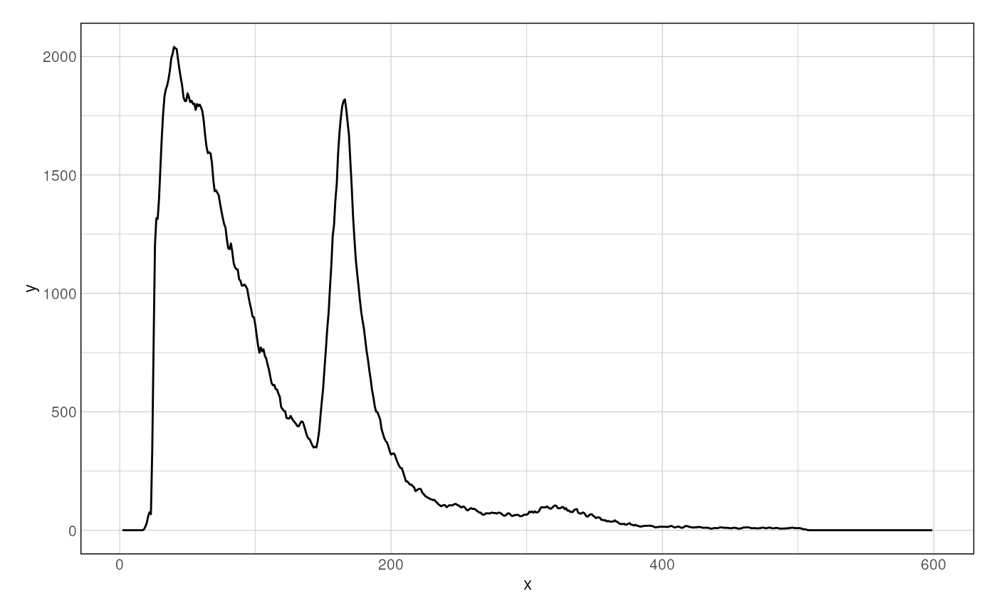
Vplot(s)
Single Vplot
Once data is imported, a V-plot of paired-end fragments over loci of
interest is generated using the plotVmat() function:
p <- plotVmat(x = MNase_sacCer3_Henikoff2011, granges = ABF1_sacCer3)
#> Computing V-mat
#> Normalizing the matrix
#> No normalization applied
#> Smoothing the matrix
p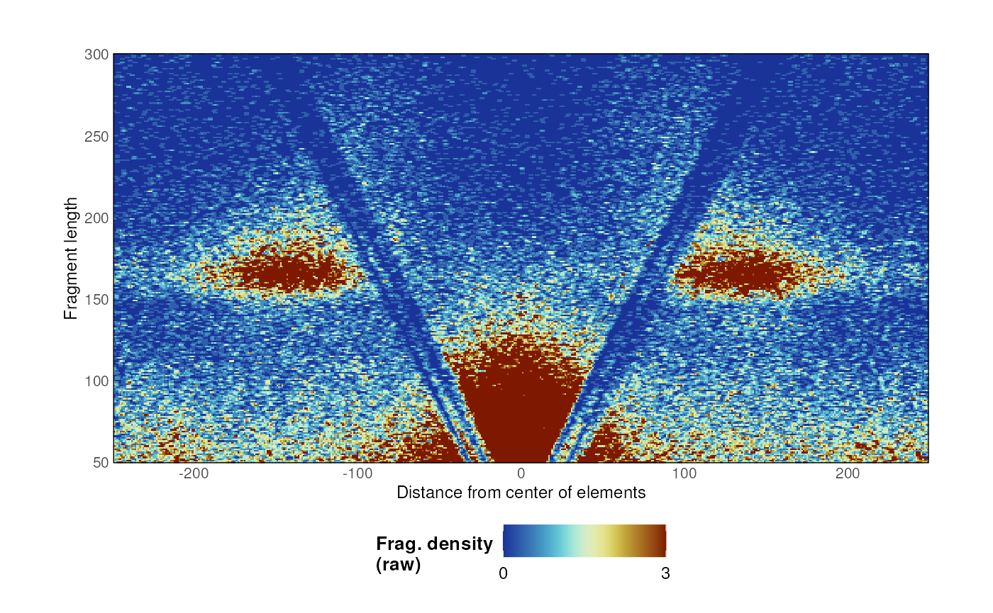
Multiple Vplots
The generation of multiple V-plots can be parallelized using a list of parameters:
list_params <- list(
    "MNase\n@ ABF1" = list(MNase_sacCer3_Henikoff2011, ABF1_sacCer3),
    "MNase\n@ random loci" = list(
        MNase_sacCer3_Henikoff2011, sampleGRanges(ABF1_sacCer3)
    )
)
p <- plotVmat(
    list_params,
    cores = 1
)
#> - Processing sample 1/2
#> - Processing sample 2/2
p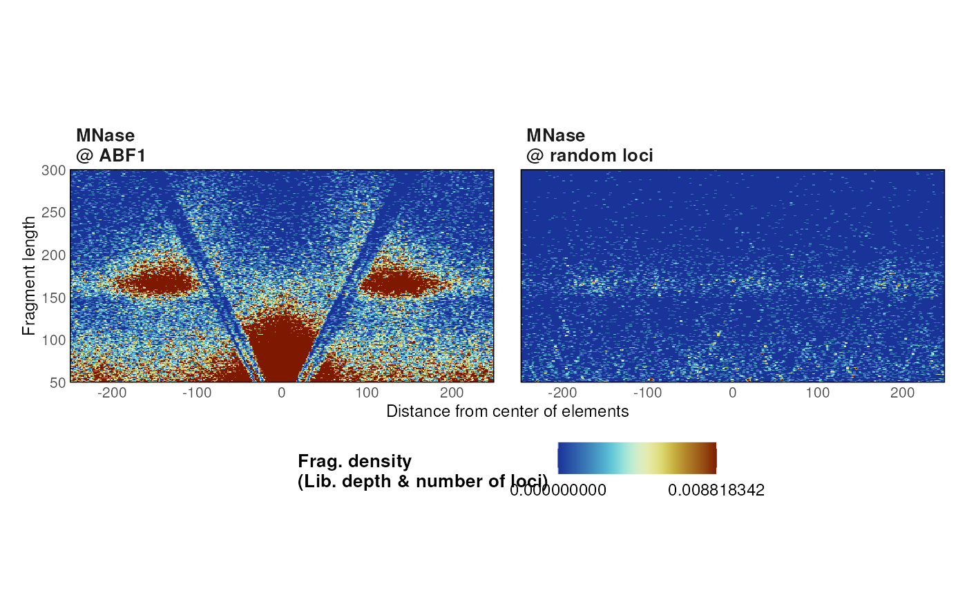
For instance, ATAC-seq fragment density can be visualized at different classes of ubiquitous and tissue-specific promoters in C. elegans.
list_params <- list(
    "Germline ATACseq\n@ Ubiq. proms" = list(
        ATAC_ce11_Serizay2020[['Germline']],
        ce11_proms[ce11_proms$which.tissues == 'Ubiq.']
    ),
    "Germline ATACseq\n@ Germline proms" = list(
        ATAC_ce11_Serizay2020[['Germline']],
        ce11_proms[ce11_proms$which.tissues == 'Germline']
    ),
    "Neuron ATACseq\n@ Ubiq. proms" = list(
        ATAC_ce11_Serizay2020[['Neurons']],
        ce11_proms[ce11_proms$which.tissues == 'Ubiq.']
    ),
    "Neuron ATACseq\n@ Neuron proms" = list(
        ATAC_ce11_Serizay2020[['Neurons']],
        ce11_proms[ce11_proms$which.tissues == 'Neurons']
    )
)
p <- plotVmat(
    list_params,
    cores = 1,
    nrow = 2, ncol = 5
)
#> - Processing sample 1/4
#> - Processing sample 2/4
#> - Processing sample 3/4
#> - Processing sample 4/4
p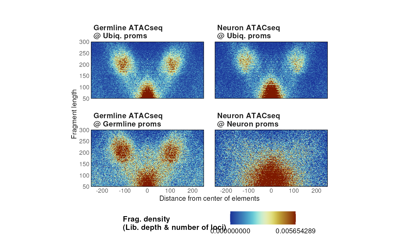
Vplots normalization
Different normalization approaches are available using the
normFun argument.
- Un-normalized raw counts can be plotted by specifying
normFun = 'none'.
# No normalization
p <- plotVmat(
    list_params,
    cores = 1,
    nrow = 2, ncol = 5,
    verbose = FALSE,
    normFun = 'none'
)
#> Computing V-mat
#> Normalizing the matrix
#> No normalization applied
#> Smoothing the matrix
#> Computing V-mat
#> Normalizing the matrix
#> No normalization applied
#> Smoothing the matrix
#> Computing V-mat
#> Normalizing the matrix
#> No normalization applied
#> Smoothing the matrix
#> Computing V-mat
#> Normalizing the matrix
#> No normalization applied
#> Smoothing the matrix
p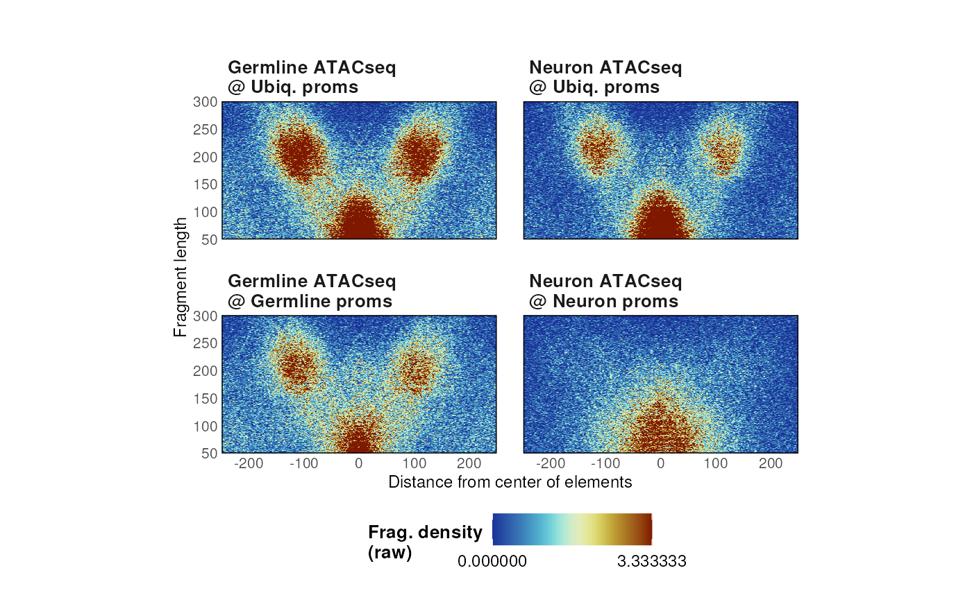
- By default, plots are normalized by the library depth of the sequencing run and by the number of loci used to compute fragment density.
# Library depth + number of loci of interest (default)
p <- plotVmat(
    list_params,
    cores = 1,
    nrow = 2, ncol = 5,
    verbose = FALSE,
    normFun = 'libdepth+nloci'
)
#> Computing V-mat
#> Normalizing the matrix
#> Computing raw library depth
#> Dividing Vmat by its number of loci
#> Smoothing the matrix
#> Computing V-mat
#> Normalizing the matrix
#> Computing raw library depth
#> Dividing Vmat by its number of loci
#> Smoothing the matrix
#> Computing V-mat
#> Normalizing the matrix
#> Computing raw library depth
#> Dividing Vmat by its number of loci
#> Smoothing the matrix
#> Computing V-mat
#> Normalizing the matrix
#> Computing raw library depth
#> Dividing Vmat by its number of loci
#> Smoothing the matrix
p
- Alternatively, heatmaps can be internally z-scored or scaled to a specific quantile.
# Zscore
p <- plotVmat(
    list_params,
    cores = 1,
    nrow = 2, ncol = 5,
    verbose = FALSE,
    normFun = 'zscore'
)
#> Computing V-mat
#> Normalizing the matrix
#> Smoothing the matrix
#> Computing V-mat
#> Normalizing the matrix
#> Smoothing the matrix
#> Computing V-mat
#> Normalizing the matrix
#> Smoothing the matrix
#> Computing V-mat
#> Normalizing the matrix
#> Smoothing the matrix
p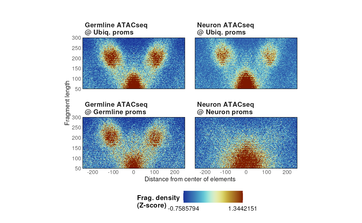
# Quantile
p <- plotVmat(
    list_params,
    cores = 1,
    nrow = 2, ncol = 5,
    verbose = FALSE,
    normFun = 'quantile',
    s = 0.99
)
#> Computing V-mat
#> Normalizing the matrix
#> Smoothing the matrix
#> Computing V-mat
#> Normalizing the matrix
#> Smoothing the matrix
#> Computing V-mat
#> Normalizing the matrix
#> Smoothing the matrix
#> Computing V-mat
#> Normalizing the matrix
#> Smoothing the matrix
p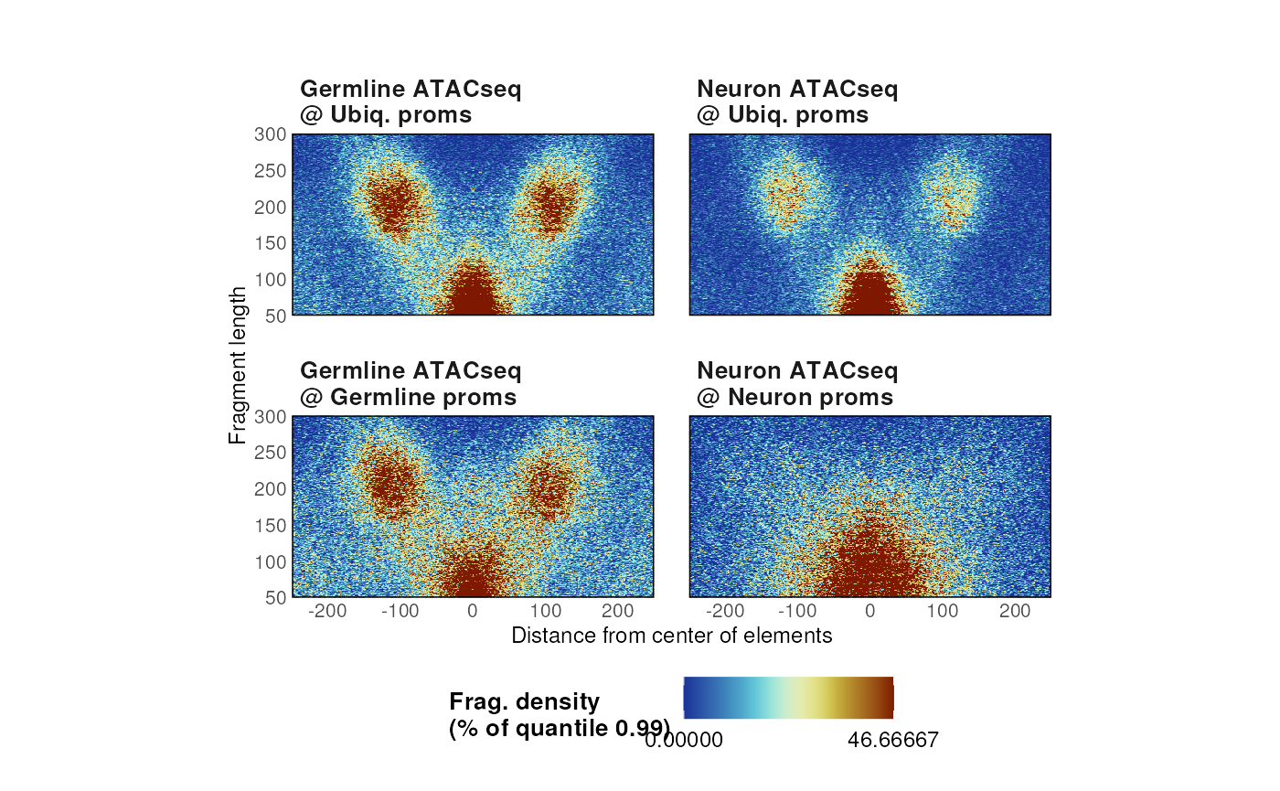
Footprints
VplotR also implements a function to profile the footprint from MNase or ATAC-seq over sets of genomic loci. For instance, CTCF is known for its ~40-bp large footprint at its binding loci.
p <- plotFootprint(
    MNase_sacCer3_Henikoff2011,
    ABF1_sacCer3
)
#> - Getting cuts
#> - Getting cut coverage
#> - Getting cut coverage / target
#> - Reformatting data into matrix
#> - Plotting footprint
p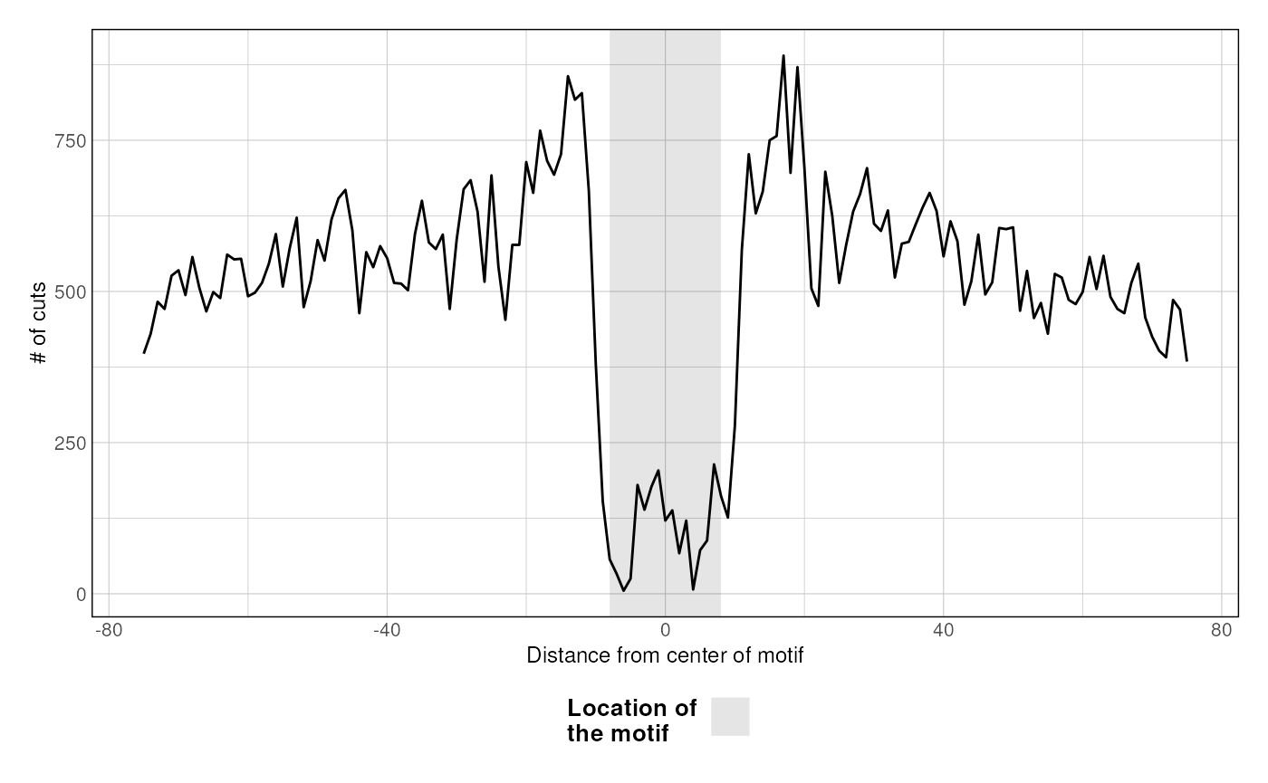
Local fragment distribution
VplotR provides a function to plot the distribution of paired-end fragments over an individual genomic window.
data(MNase_sacCer3_Henikoff2011_subset)
genes_sacCer3 <- GenomicFeatures::genes(TxDb.Scerevisiae.UCSC.sacCer3.sgdGene::
    TxDb.Scerevisiae.UCSC.sacCer3.sgdGene
)
p <- plotProfile(
    fragments = MNase_sacCer3_Henikoff2011_subset,
    window = "chrXV:186,400-187,400",
    loci = ABF1_sacCer3,
    annots = genes_sacCer3,
    min = 20, max = 200, alpha = 0.1, size = 1.5
)
#> Filtering and resizing fragments
#> 32276 fragments mapped over 1001 bases
#> Filtering and resizing fragments
#> Generating plot
#> Warning: Removed 49 rows containing missing values (`geom_line()`).
#> Warning: Removed 5176 rows containing missing values (`geom_point()`).
#> Warning: Removed 19 rows containing missing values (`geom_line()`).
p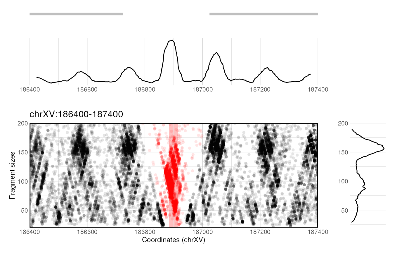
Session Info
sessionInfo()
#> R Under development (unstable) (2023-11-22 r85609)
#> Platform: x86_64-pc-linux-gnu
#> Running under: Ubuntu 22.04.3 LTS
#>
#> Matrix products: default
#> BLAS:   /usr/lib/x86_64-linux-gnu/openblas-pthread/libblas.so.3
#> LAPACK: /usr/lib/x86_64-linux-gnu/openblas-pthread/libopenblasp-r0.3.20.so;  LAPACK version 3.10.0
#>
#> locale:
#>  [1] LC_CTYPE=en_US.UTF-8       LC_NUMERIC=C
#>  [3] LC_TIME=en_US.UTF-8        LC_COLLATE=en_US.UTF-8
#>  [5] LC_MONETARY=en_US.UTF-8    LC_MESSAGES=en_US.UTF-8
#>  [7] LC_PAPER=en_US.UTF-8       LC_NAME=C
#>  [9] LC_ADDRESS=C               LC_TELEPHONE=C
#> [11] LC_MEASUREMENT=en_US.UTF-8 LC_IDENTIFICATION=C
#>
#> time zone: UTC
#> tzcode source: system (glibc)
#>
#> attached base packages:
#> [1] stats4    stats     graphics  grDevices utils     datasets  methods
#> [8] base
#>
#> other attached packages:
#> [1] VplotR_1.12.1        ggplot2_3.4.4        GenomicRanges_1.55.1
#> [4] GenomeInfoDb_1.39.1  IRanges_2.37.0       S4Vectors_0.41.2
#> [7] BiocGenerics_0.49.1
#>
#> loaded via a namespace (and not attached):
#>   [1] DBI_1.1.3
#>   [2] bitops_1.0-7
#>   [3] biomaRt_2.59.0
#>   [4] rlang_1.1.2
#>   [5] magrittr_2.0.3
#>   [6] matrixStats_1.1.0
#>   [7] compiler_4.4.0
#>   [8] RSQLite_2.3.3
#>   [9] GenomicFeatures_1.55.1
#>  [10] png_0.1-8
#>  [11] systemfonts_1.0.5
#>  [12] vctrs_0.6.4
#>  [13] reshape2_1.4.4
#>  [14] stringr_1.5.1
#>  [15] pkgconfig_2.0.3
#>  [16] crayon_1.5.2
#>  [17] fastmap_1.1.1
#>  [18] dbplyr_2.4.0
#>  [19] XVector_0.43.0
#>  [20] labeling_0.4.3
#>  [21] utf8_1.2.4
#>  [22] Rsamtools_2.19.2
#>  [23] rmarkdown_2.25
#>  [24] ragg_1.2.6
#>  [25] purrr_1.0.2
#>  [26] bit_4.0.5
#>  [27] xfun_0.41
#>  [28] zlibbioc_1.49.0
#>  [29] cachem_1.0.8
#>  [30] jsonlite_1.8.7
#>  [31] progress_1.2.2
#>  [32] blob_1.2.4
#>  [33] highr_0.10
#>  [34] DelayedArray_0.29.0
#>  [35] BiocParallel_1.37.0
#>  [36] parallel_4.4.0
#>  [37] prettyunits_1.2.0
#>  [38] R6_2.5.1
#>  [39] bslib_0.6.1
#>  [40] stringi_1.8.2
#>  [41] RColorBrewer_1.1-3
#>  [42] rtracklayer_1.63.0
#>  [43] jquerylib_0.1.4
#>  [44] Rcpp_1.0.11
#>  [45] SummarizedExperiment_1.33.1
#>  [46] knitr_1.45
#>  [47] zoo_1.8-12
#>  [48] Matrix_1.6-3
#>  [49] tidyselect_1.2.0
#>  [50] abind_1.4-5
#>  [51] yaml_2.3.7
#>  [52] codetools_0.2-19
#>  [53] curl_5.1.0
#>  [54] lattice_0.22-5
#>  [55] tibble_3.2.1
#>  [56] plyr_1.8.9
#>  [57] Biobase_2.63.0
#>  [58] withr_2.5.2
#>  [59] KEGGREST_1.43.0
#>  [60] evaluate_0.23
#>  [61] desc_1.4.2
#>  [62] BiocFileCache_2.11.1
#>  [63] xml2_1.3.5
#>  [64] Biostrings_2.71.1
#>  [65] filelock_1.0.2
#>  [66] pillar_1.9.0
#>  [67] MatrixGenerics_1.15.0
#>  [68] generics_0.1.3
#>  [69] rprojroot_2.0.4
#>  [70] RCurl_1.98-1.13
#>  [71] hms_1.1.3
#>  [72] munsell_0.5.0
#>  [73] scales_1.3.0
#>  [74] glue_1.6.2
#>  [75] tools_4.4.0
#>  [76] BiocIO_1.13.0
#>  [77] GenomicAlignments_1.39.0
#>  [78] fs_1.6.3
#>  [79] XML_3.99-0.16
#>  [80] cowplot_1.1.1
#>  [81] grid_4.4.0
#>  [82] TxDb.Scerevisiae.UCSC.sacCer3.sgdGene_3.2.2
#>  [83] AnnotationDbi_1.65.2
#>  [84] colorspace_2.1-0
#>  [85] GenomeInfoDbData_1.2.11
#>  [86] restfulr_0.0.15
#>  [87] cli_3.6.1
#>  [88] rappdirs_0.3.3
#>  [89] textshaping_0.3.7
#>  [90] fansi_1.0.5
#>  [91] S4Arrays_1.3.1
#>  [92] dplyr_1.1.4
#>  [93] gtable_0.3.4
#>  [94] sass_0.4.7
#>  [95] digest_0.6.33
#>  [96] SparseArray_1.3.1
#>  [97] rjson_0.2.21
#>  [98] farver_2.1.1
#>  [99] memoise_2.0.1
#> [100] htmltools_0.5.7
#> [101] pkgdown_2.0.7
#> [102] lifecycle_1.0.4
#> [103] httr_1.4.7
#> [104] bit64_4.0.5