Session 2: from clusters to cell types
Jacques Serizay
2026-09-02
Source:vignettes/c_session2.Rmd
c_session2.RmdGoals of this session
Last week we turned a text file into a map of 5.5K cells. Today we put names on it.
| # | Step | Time |
|---|---|---|
| 0 | Getting your object back | 4 min |
| 1 | Clustering | 12 min |
| 2 | Visualising and sanity-checking clusters | 10 min |
| 3 | Manually checking known markers | 10 min |
| 4 | Annotating automatically, against a public reference | 15 min |
| 5 | Real differential expression: pseudobulk and
DESeq2
|
8 min |
0. Getting your object back
Load the packages we will need today. Nothing here is new: these are
the same libraries as last week, plus bluster for
clustering and SingleR/celldex for
annotation:
library(SingleCellExperiment)
library(Matrix)
library(scuttle)
library(scran)
library(scater)
library(bluster)
library(ggplot2)
Session 1 ended with saveRDS().
sce_path <- "path_to_your_sce.rds"
sce <- readRDS(sce_path)
If you lost the file, the code below can recover the same object from the workshop package.
Everything is where we left it: counts, logcounts, cell metadata, PCA and UMAP for logcounts and batch-corrected data. We are ready to cluster and annotate.
sce
#> class: SingleCellExperiment
#> dim: 27477 5583
#> metadata(1): qc
#> assays(2): counts logcounts
#> rownames(27477): RP11-34P13.3 RP11-34P13.7 ... AC136612.1 AC145212.4
#> rowData names(0):
#> colnames: NULL
#> colData names(9): Donor Barcode ... keep sizeFactor
#> reducedDimNames(4): PCA UMAP corrected UMAP_corrected
#> mainExpName: NULL
#> altExpNames(0):
1. Clustering
This is the step where single-cell analysis stops looking like bulk. In bulk you know your groups: treated and untreated, tumour and normal. Here the groups are what you are trying to find.
The standard Bioconductor approach is graph-based clustering:
- build a graph where each cell is connected to its k nearest neighbours in PCA space;
- weight the edges by how many neighbours two cells share;
- hand the graph to a community-detection algorithm (Louvain, Leiden, walktrap) which cuts it into densely connected groups.
It scales to millions of cells, makes no assumption about cluster shape, and has exactly one parameter that matters: k.
We decided last week to work with the first 20 PCs. A
reducedDim is just a matrix, so pull them out:
pcs <- reducedDim(sce, "PCA")[, 1:20]
dim(pcs)
#> [1] 5583   20
bluster::clusterRows() clusters the rows of any matrix.
You hand it the data and a parameter object saying which
algorithm to use — here, a nearest neighbour graph with Louvain
community detection:
set.seed(2026)
sce$cluster <- clusterRows(pcs, NNGraphParam(k = 20, cluster.fun = "louvain"))
table(sce$cluster)
#>
#>   1   2   3   4   5   6   7   8   9  10  11  12  13  14  15
#> 630 528 465 455 247 284 472 329 330 316 320 172 327 391 317
You will also see
scran::clusterCells(sce, use.dimred = "PCA") in OSCA and in
older tutorials. It is a convenience wrapper that calls
clusterRows() for you; on recent Bioconductor it is
deprecated in favour of calling clusterRows() directly,
which is what we do here.
k is a resolution dial, not a truth setting
Small k gives a sparse graph and many small communities;
large k gives a dense graph and few large ones. There is no
correct value — there is only the resolution at which the
biology you care about becomes visible.
ks <- c(5, 10, 20, 50)
n_clusters <- vapply(ks, function(k) {
    set.seed(2026)
    nlevels(clusterRows(pcs, NNGraphParam(k = k, cluster.fun = "louvain")))
}, integer(1))

data.frame(k = ks, clusters = n_clusters)
#>    k clusters
#> 1  5       24
#> 2 10       19
#> 3 20       15
#> 4 50       13
Do not go looking for the “right” number of clusters. Pick a resolution, annotate it, and check whether the populations you can name are separated. If two clusters have the same markers, merge them. If one cluster obviously contains two cell types, split it. Clustering is a tool for generating hypotheses, not a measurement.
2. Visualising and sanity-checking clusters
plotUMAP(sce, dimred = "UMAP_corrected", colour_by = "cluster", text_by = "cluster")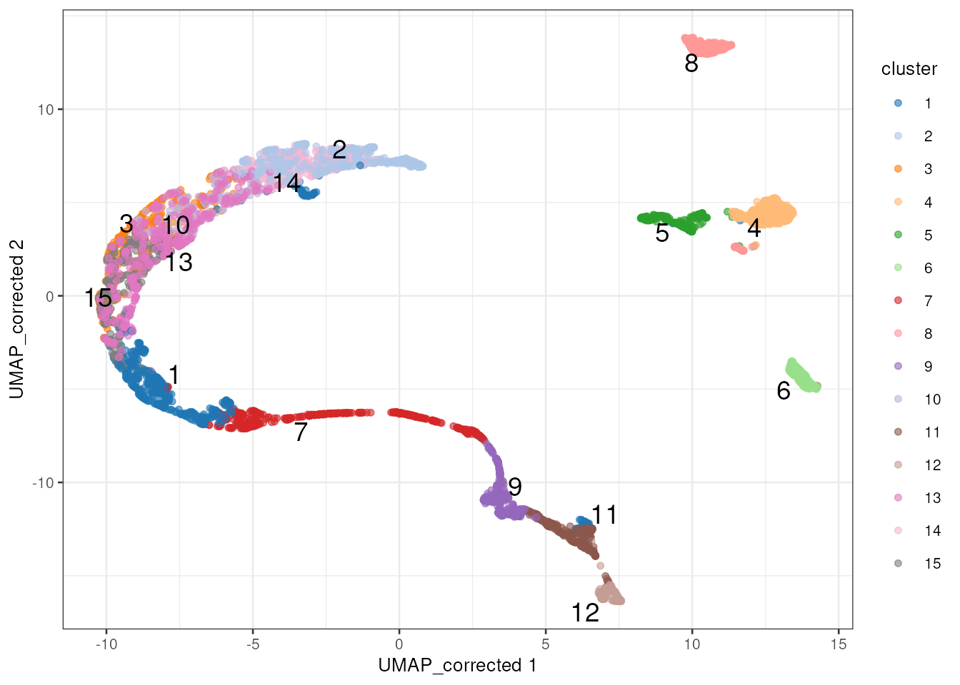
Two questions to ask of any clustering, in this order.
Are the clusters shared between donors, or did I just cluster by individual?
tab <- table(Cluster = sce$cluster, Sample = sce$Sample)
tab
#>        Sample
#> Cluster Donor1_rep1 Donor1_rep2 Donor2_rep1 Donor2_rep2 Donor3_rep1 Donor3_rep2
#>      1           45          77         180         145          87          96
#>      2          108         172         113         114           9          12
#>      3            0           0         209         253           2           1
#>      4          132         135          74           4          44          66
#>      5           96          20          80          33          12           6
#>      6           75          58          58          11          47          35
#>      7           33          83          68          95          97          96
#>      8          154          67          35           3          41          29
#>      9          102         182          10           0           2          34
#>      10           0           0           2           1         147         166
#>      11         103         164           7           0          11          35
#>      12          35          94          10           3           8          22
#>      13         116         196           3           4           4           4
#>      14           1           0           0           0         188         202
#>      15           0           0           0           0         158         159

ggplot(as.data.frame(tab), aes(x = Cluster, y = Freq, fill = Sample)) +
    geom_col(position = "fill") +
    labs(y = "Proportion of cells", x = "Cluster") +
    theme_bw()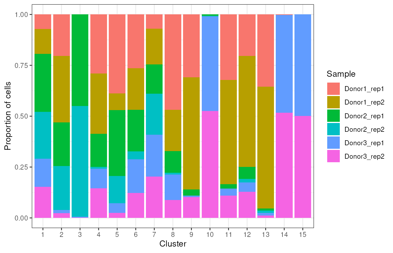
A cluster that does not have all colours is suspect: it may come from a technical batch effect rather than a biological population. Alternatively, it could be a rare population that is only present in one donor. You will need to check the markers to decide!
3. Annotating by hand, with known markers
Clusters are numbers. Biology needs names. The most reliable way to get from one to the other is still a panel of genes you trust from the literature:
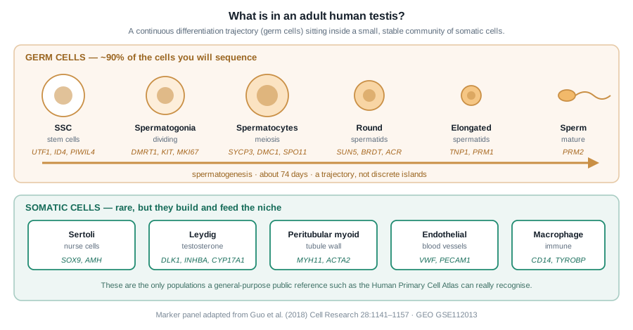
panels <- list(
    SSC             = c("UTF1", "ID4", "PIWIL4"),
    Spermatogonia   = c("DMRT1", "KIT", "MKI67"),
    Spermatocyte    = c("SYCP3", "DMC1", "SPO11"),
    RoundSpermatid  = c("SUN5", "ACR", "BRDT"),
    ElongSpermatid  = c("TNP1", "PRM1", "PRM2"),
    Sertoli         = c("SOX9", "AMH"),
    Leydig          = c("DLK1", "INHBA", "CYP17A1"),
    Myoid           = c("MYH11", "ACTA2"),
    Endothelial     = c("VWF", "PECAM1"),
    Macrophage      = c("CD14", "TYROBP")
)
plotDots(sce, features = unique(unlist(panels)), group = "cluster") +
    theme(axis.text.x = element_text(angle = 45, hjust = 1))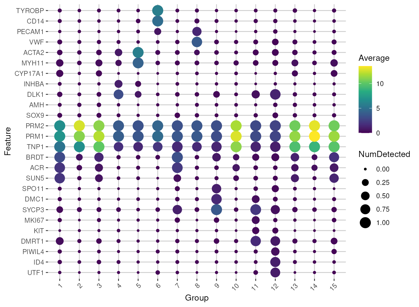
- Dot size is the fraction of cells in the cluster expressing the gene;
- Dot colour is the average expression among them. Read down each column and the cluster names write themselves.
plotUMAP(sce, dimred = "UMAP_corrected", colour_by = "TNP1", text_by = "cluster")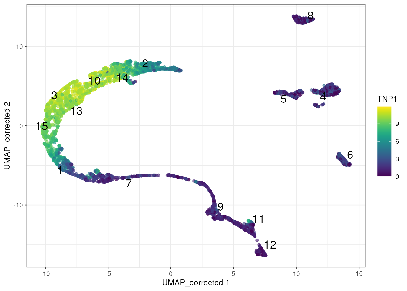
In real life, you now stare at the dot plot and type
annotations <- c("1" = "Sertoli", "2" = "Spermatocyte", ...).
That breaks the moment the clustering changes (eg if you re-run the
analysis with a different seed, or a different k).
4. Annotating automatically, against a public reference
Hand annotation does not scale, and it only finds what you already thought to look for. The alternative is to compare each cell with a published reference of labelled expression profiles.
SingleR does this by correlating each cell against the
reference profiles, using only genes that discriminate between reference
labels, then repeatedly discarding the worst-scoring labels until one
wins.
We are going to use a pre-computed scRNAseq reference atlas from the Human Protein Atlas, provided in this workshop.
data("HPA_ref", package = "BiocAfricaScRNAseq2026")
HPA_ref
#> class: SummarizedExperiment
#> dim: 20151 154
#> metadata(0):
#> assays(1): logcounts
#> rownames(20151): TSPAN6 TNMD ... ENSG00000291316 TMEM276
#> rowData names(0):
#> colnames(154): adipocytes adrenal cortex cells ... vascular endothelial
#>   cells vascular smooth muscle cells
#> colData names(1): label
The HPA reference is a scRNAseq atlas of many human tissues. It is not however specifically focusing on testis, and its germ-cell representation may be coarse. Look at what labels are actually on offer:
length(unique(HPA_ref$label))
#> [1] 154
sort(unique(HPA_ref$label))
#>   [1] "adipocytes"
#>   [2] "adrenal cortex cells"
#>   [3] "adrenal medulla cells"
#>   [4] "alveolar cells type 1"
#>   [5] "alveolar cells type 2"
#>   [6] "astrocytes"
#>   [7] "b-cells"
#>   [8] "basal keratinocytes"
#>   [9] "basal prostatic cells"
#>  [10] "bergmann glia"
#>  [11] "brain excitatory neurons"
#>  [12] "brain inhibitory neurons"
#>  [13] "breast hormone-responsive cells"
#>  [14] "breast lactating cells"
#>  [15] "breast myoepithelial cells"
#>  [16] "breast secretory cells"
#>  [17] "cardiomyocytes"
#>  [18] "cdc"
#>  [19] "cholangiocytes"
#>  [20] "choroid plexus epithelial cells"
#>  [21] "colonocytes"
#>  [22] "cone photoreceptor cells"
#>  [23] "conjunctival goblet cells"
#>  [24] "corticotrophs"
#>  [25] "cytotrophoblasts"
#>  [26] "decidual stromal cells"
#>  [27] "differentiating spermatogonia"
#>  [28] "distal convoluted tubule cells"
#>  [29] "early primary spermatocytes"
#>  [30] "early spermatids"
#>  [31] "endometrial ciliated cells"
#>  [32] "endometrial glandular cells"
#>  [33] "endometrial luminal cells"
#>  [34] "endometrial secretory cells"
#>  [35] "endometrial stromal cells"
#>  [36] "enteric stem cells"
#>  [37] "enteric transient amplifying cells"
#>  [38] "enterocytes"
#>  [39] "ependymal cells"
#>  [40] "epicardial cells"
#>  [41] "epididymal basal cells"
#>  [42] "epididymal clear cells"
#>  [43] "epididymal efferent duct absorptive cells"
#>  [44] "epididymal efferent duct ciliated cells"
#>  [45] "epididymal principal cells"
#>  [46] "erythrocyte progenitors"
#>  [47] "erythrocytes"
#>  [48] "esophageal apical cells"
#>  [49] "esophageal basal cells"
#>  [50] "esophageal suprabasal cells"
#>  [51] "extravillous trophoblasts"
#>  [52] "fallopian secretory cells"
#>  [53] "fallopian tube ciliated cells"
#>  [54] "fibro-adipogenic progenitors"
#>  [55] "fibroblasts"
#>  [56] "foveolar cells"
#>  [57] "gastric chief cells"
#>  [58] "gastric progenitor cells"
#>  [59] "goblet cells"
#>  [60] "gonadotrophs"
#>  [61] "granulosa cells"
#>  [62] "hematopoietic stem cells"
#>  [63] "hepatic stellate cells"
#>  [64] "hepatocytes"
#>  [65] "hofbauer cells"
#>  [66] "innate lymphoid cells"
#>  [67] "kupffer cells"
#>  [68] "lacrimal acinar cells"
#>  [69] "lactotrophs"
#>  [70] "late primary spermatocytes"
#>  [71] "late spermatids"
#>  [72] "leydig cells"
#>  [73] "loop of henle epithelial cells"
#>  [74] "lymphatic endothelial cells"
#>  [75] "macrophages"
#>  [76] "mast cells"
#>  [77] "medullary thymic epithelial cells"
#>  [78] "megakaryocyte progenitors"
#>  [79] "megakaryocyte-erythroid progenitors"
#>  [80] "megakaryocytes"
#>  [81] "melanocytes"
#>  [82] "mesothelial cells"
#>  [83] "microglia"
#>  [84] "migrating cytotrophoblasts"
#>  [85] "monocyte progenitors"
#>  [86] "monocytes"
#>  [87] "mucous neck cells"
#>  [88] "müller glia"
#>  [89] "myonuclei"
#>  [90] "myosatellite cells"
#>  [91] "neuroendocrine cells"
#>  [92] "neutrophil progenitors"
#>  [93] "neutrophils"
#>  [94] "nk-cells"
#>  [95] "ocular epithelial cells"
#>  [96] "oligodendrocyte progenitor cells"
#>  [97] "oligodendrocytes"
#>  [98] "oocytes"
#>  [99] "other brain neurons"
#> [100] "ovarian stromal cells"
#> [101] "pancreatic acinar cells"
#> [102] "pancreatic duct cells"
#> [103] "pancreatic islet cells"
#> [104] "paneth cells"
#> [105] "papillary tip epithelial cells"
#> [106] "parietal cells"
#> [107] "pdcs"
#> [108] "pericytes"
#> [109] "peritubular myoid cells"
#> [110] "pituicytes/fscs"
#> [111] "pituitary stem cells"
#> [112] "plasma cells"
#> [113] "platelets"
#> [114] "podocytes"
#> [115] "prostatic club cells"
#> [116] "prostatic glandular cells"
#> [117] "prostatic hillock cells"
#> [118] "proximal tubule cells"
#> [119] "renal collecting duct intercalated cells"
#> [120] "renal collecting duct principal cells"
#> [121] "renal connecting tubule cells"
#> [122] "respiratory basal cells"
#> [123] "respiratory ciliated cells"
#> [124] "respiratory deuterosomal cells"
#> [125] "respiratory ionocytes"
#> [126] "respiratory secretory cells"
#> [127] "retinal amacrine cells"
#> [128] "retinal bipolar cells"
#> [129] "retinal ganglion cells"
#> [130] "retinal horizontal cells"
#> [131] "retinal pigment epithelial cells"
#> [132] "rod photoreceptor cells"
#> [133] "salivary acinar cells"
#> [134] "salivary basal cells"
#> [135] "salivary duct cells"
#> [136] "salivary ionocytes"
#> [137] "salivary myoepithelial cells"
#> [138] "schwann cells"
#> [139] "sertoli cells"
#> [140] "smooth muscle cells"
#> [141] "somatotrophs"
#> [142] "submucosal glandular cells"
#> [143] "suprabasal keratinocytes"
#> [144] "syncytiotrophoblasts"
#> [145] "t-cells"
#> [146] "thymic myoid cells"
#> [147] "thymocytes"
#> [148] "thyrotrophs"
#> [149] "transitional alveolar cells"
#> [150] "tuft cells"
#> [151] "undifferentiated spermatogonia"
#> [152] "urothelial cells"
#> [153] "vascular endothelial cells"
#> [154] "vascular smooth muscle cells"
Passing clusters= makes SingleR pool the
cells of each cluster first and label the cluster as a whole. This is
more robust than labelling single cells, because a pooled profile is far
less noisy:
library(SingleR)
pred_cluster <- SingleR(
    test     = sce,
    ref      = HPA_ref,
    labels   = HPA_ref$label,
    clusters = sce$cluster
)
sce$celltype <- factor(pred_cluster$labels[sce$cluster])
plotUMAP(sce, dimred = "UMAP_corrected", colour_by = "celltype", text_by = "celltype")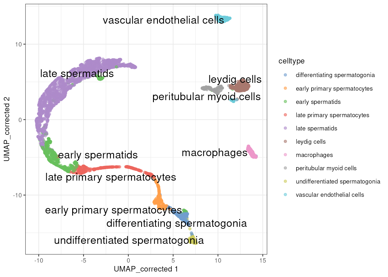
Two things we can observe in this map:
- The germ-cell labels should lie along one continuous arc, in
developmental order: spermatogenesis is a trajectory, and
clustering has cut it into segments whose boundaries are a consequence
of
k, not of biology. - The somatic labels should sit apart as genuinely discrete populations. Trust the boundaries in the second case; do not over-interpret them in the first.
5. Real differential expression: pseudobulk and
DESeq2
When it comes to testing for differential expression, we cannot test between celltypes that we defined from the same data. So what can we test?
The rule is short: your unit of replication is the sample, not the cell. Three donors give you n = 3, whether you sequenced 600 cells or 600,000. Two cells from the same donor are not independent observations.
The standard solution is pseudobulk: sum the counts of all cells of one type within one sample, giving you back a small bulk-like matrix — and then use the tools you already know from the introductory workshop.
pbulk <- aggregateAcrossCells(
    sce,
    ids = colData(sce)[, c("celltype", "Sample")],
    use.assay.type = "counts"
)
pbulk
#> class: SingleCellExperiment
#> dim: 27477 58
#> metadata(1): qc
#> assays(1): counts
#> rownames(27477): RP11-34P13.3 RP11-34P13.7 ... AC136612.1 AC145212.4
#> rowData names(0):
#> colnames: NULL
#> colData names(14): Donor Barcode ... Sample ncells
#> reducedDimNames(4): PCA UMAP corrected UMAP_corrected
#> mainExpName: NULL
#> altExpNames(0):
pbulk$Donor <- sub("_rep.*$", "", pbulk$Sample)
head(data.frame(celltype = pbulk$celltype, Sample = pbulk$Sample, ncells = pbulk$ncells))
#>                        celltype      Sample ncells
#> 1 differentiating spermatogonia Donor1_rep1    103
#> 2 differentiating spermatogonia Donor1_rep2    164
#> 3 differentiating spermatogonia Donor2_rep1      7
#> 4 differentiating spermatogonia Donor3_rep1     11
#> 5 differentiating spermatogonia Donor3_rep2     35
#> 6   early primary spermatocytes Donor1_rep1    102
Each column is now one celltype in one sample. We contrast two large-ish celltype clusters, blocking on donor:
pbulk2  <- pbulk[, pbulk$celltype %in% c("undifferentiated spermatogonia", "late spermatids")]
table(celltype = as.character(pbulk2$celltype), donor = pbulk2$Donor)
#>                                 donor
#> celltype                         Donor1 Donor2 Donor3
#>   late spermatids                     2      2      2
#>   undifferentiated spermatogonia      2      2      2
We can now convert this into a DESeqDataSet and run the
same analysis we did in the pre-workshop refresher.
library(DESeq2)
se <- as(pbulk2, "SummarizedExperiment")
rownames(se) <- rownames(pbulk2)
se$sizeFactor <- NULL
dds <- DESeqDataSet(se, design = ~ Donor + celltype)
dim(dds)
#> [1] 27477    12
That is the same DESeqDataSet you built in the
pre-workshop refresher, from the same kind of design formula. Nothing
about the fitting changes:
dds <- DESeq(dds)
res <- results(dds, c("celltype", "late spermatids", "undifferentiated spermatogonia"))
summary(res)
#>
#> out of 26356 with nonzero total read count
#> adjusted p-value < 0.1
#> LFC > 0 (up)       : 10057, 38%
#> LFC < 0 (down)     : 6119, 23%
#> outliers [1]       : 0, 0%
#> low counts [2]     : 4079, 15%
#> (mean count < 0)
#> [1] see 'cooksCutoff' argument of ?results
#> [2] see 'independentFiltering' argument of ?results
Let’s look at the top hits. We can filter for a log2 fold change of at least 2 and sort by adjusted p-value.
res |>
    dplyr::as_tibble(rownames = "gene") |>
    dplyr::filter(log2FoldChange >= 2) |>
    dplyr::arrange(padj)
#> # A tibble: 8,084 × 7
#>    gene      baseMean log2FoldChange  lfcSE  stat pvalue  padj
#>    <chr>        <dbl>          <dbl>  <dbl> <dbl>  <dbl> <dbl>
#>  1 HMGB4        8554.           8.99 0.191   47.1      0     0
#>  2 GSTM3        1319.           5.70 0.116   49.1      0     0
#>  3 SMCP         4181.           8.34 0.208   40.2      0     0
#>  4 LELP1        6212.           8.98 0.174   51.5      0     0
#>  5 TSACC        5881.           7.51 0.117   64.4      0     0
#>  6 MPC2         1795.           5.19 0.118   44.1      0     0
#>  7 GLUL         2603.           6.52 0.167   39.1      0     0
#>  8 LINC00467    6712.           6.63 0.0881  75.2      0     0
#>  9 CEP170       1681.           7.52 0.176   42.8      0     0
#> 10 TNP1        49841.           9.92 0.124   79.7      0     0
#> # ℹ 8,074 more rows
plotUMAP(sce, dimred = "UMAP_corrected", colour_by = "GLUL", text_by = "celltype")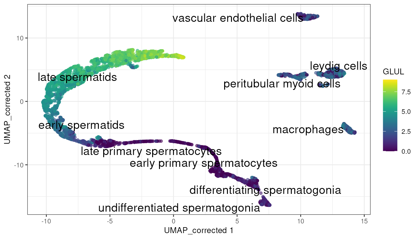
Exercises
1. Recluster with k = 5
(clusterRows(pcs, NNGraphParam(k = 5, cluster.fun = "louvain")))
and store it as sce$cluster_fine. Cross-tabulate against
sce$celltype. Which of your annotated populations split
into several fine clusters — and can you find markers that distinguish
the pieces?
2. Build the pseudobulk matrix per cell
type rather than per cluster and run DESeq2 on it.
How many genes are differentially expressed between clusters 2 and
4?
sessionInfo()
#> R version 4.6.0 (2026-04-24)
#> Platform: x86_64-pc-linux-gnu
#> Running under: Ubuntu 24.04.4 LTS
#>
#> Matrix products: default
#> BLAS:   /usr/lib/x86_64-linux-gnu/openblas-pthread/libblas.so.3
#> LAPACK: /usr/lib/x86_64-linux-gnu/openblas-pthread/libopenblasp-r0.3.26.so;  LAPACK version 3.12.0
#>
#> locale:
#>  [1] LC_CTYPE=en_US.UTF-8       LC_NUMERIC=C
#>  [3] LC_TIME=en_US.UTF-8        LC_COLLATE=en_US.UTF-8
#>  [5] LC_MONETARY=en_US.UTF-8    LC_MESSAGES=en_US.UTF-8
#>  [7] LC_PAPER=en_US.UTF-8       LC_NAME=C
#>  [9] LC_ADDRESS=C               LC_TELEPHONE=C
#> [11] LC_MEASUREMENT=en_US.UTF-8 LC_IDENTIFICATION=C
#>
#> time zone: Etc/UTC
#> tzcode source: system (glibc)
#>
#> attached base packages:
#> [1] stats4    stats     graphics  grDevices utils     datasets  methods
#> [8] base
#>
#> other attached packages:
#>  [1] DESeq2_1.53.2               SingleR_2.15.3
#>  [3] bluster_1.23.1              scater_1.41.2
#>  [5] ggplot2_4.0.3               scran_1.41.1
#>  [7] scuttle_1.23.2              Matrix_1.7-6
#>  [9] SingleCellExperiment_1.35.2 SummarizedExperiment_1.43.0
#> [11] Biobase_2.73.2              GenomicRanges_1.65.1
#> [13] Seqinfo_1.3.2               IRanges_2.47.5
#> [15] S4Vectors_0.51.9            BiocGenerics_0.59.12
#> [17] generics_0.1.4              MatrixGenerics_1.25.0
#> [19] matrixStats_1.5.0
#>
#> loaded via a namespace (and not attached):
#>  [1] tidyselect_1.2.1    viridisLite_0.4.3   dplyr_1.2.1
#>  [4] vipor_0.4.7         farver_2.1.2        viridis_0.6.5
#>  [7] S7_0.2.2            fastmap_1.2.0       scrapper_1.7.9
#> [10] digest_0.6.39       rsvd_1.0.5          lifecycle_1.0.5
#> [13] cluster_2.1.8.3     statmod_1.5.2       magrittr_2.0.5
#> [16] compiler_4.6.0      rlang_1.3.0         sass_0.4.10
#> [19] tools_4.6.0         utf8_1.2.6          igraph_2.3.3
#> [22] yaml_2.3.12         knitr_1.51          labeling_0.4.3
#> [25] S4Arrays_1.13.0     dqrng_0.4.1         htmlwidgets_1.6.4
#> [28] DelayedArray_0.39.6 RColorBrewer_1.1-3  abind_1.4-8
#> [31] BiocParallel_1.47.0 withr_3.0.3         desc_1.4.3
#> [34] grid_4.6.0          beachmat_2.29.2     edgeR_4.99.1
#> [37] scales_1.4.0        cli_3.6.6           rmarkdown_2.32
#> [40] ragg_1.5.2          otel_0.2.0          metapod_1.21.0
#> [43] ggbeeswarm_0.7.3    cachem_1.1.0        parallel_4.6.0
#> [46] XVector_0.53.0      vctrs_0.7.3         jsonlite_2.0.0
#> [49] BiocSingular_1.29.1 BiocNeighbors_2.7.3 ggrepel_0.9.8
#> [52] irlba_2.3.7         beeswarm_0.4.0      systemfonts_1.3.2
#> [55] locfit_1.5-9.12     limma_3.99.0        jquerylib_0.1.4
#> [58] glue_1.8.1          pkgdown_2.2.1       codetools_0.2-20
#> [61] gtable_0.3.6        ScaledMatrix_1.21.0 tibble_3.3.1
#> [64] pillar_1.11.1       htmltools_0.5.9     R6_2.6.1
#> [67] textshaping_1.0.5   evaluate_1.0.5      lattice_0.23-1
#> [70] bslib_0.12.0        Rcpp_1.1.2          gridExtra_2.3.1
#> [73] SparseArray_1.13.2  xfun_0.60           fs_2.1.0
#> [76] pkgconfig_2.0.3