0. Before you start

Setup, data download, and a refresher on what you already know

Jacques Serizay

2026-09-02

Work through this page on your own, before Day 1. It takes about 45 minutes. Nothing here is taught live: the two sessions start from the assumption that your machine is ready and that the words SummarizedExperiment, assay() and colData() mean something to you.

---

Goals of the workshop

• Read a plain count matrix into R and wrap it in a SingleCellExperiment.
• Run the standard Bioconductor pre-processing workflow: quality control, normalisation, feature selection, dimensionality reduction.
• Cluster cells and visualise them on a UMAP.
• Find the genes that mark each cluster, and read the output critically.
• Annotate clusters against a public reference with SingleR.

Tips

• Type the code, do not paste it. You will remember logNormCounts() because your fingers typed it, not because you copied it. Typos are part of the lesson: you will see the error message and learn what it means.
• Say when you are stuck, immediately. Use the chat. A helper will answer while the session continues. Do not wait until the end.
• If you fall behind, stop typing and watch. It’s better to see the next step than to be stuck on the previous one.
• Everything is saved to disk at the end of Session 1 and reloaded at the start of Session 2, so you do not have to keep R open for a week.

What you should already know

You should be comfortable with the material of the introductory Bioconductor workshop:

• what a SummarizedExperiment is, and how to reach inside it;
• roughly what DESeq2 does to a bulk RNA-seq count matrix.

Step 1 and Step 2 below are a short refresher on those two points. If they feel easy, you are ready.

---

The dataset

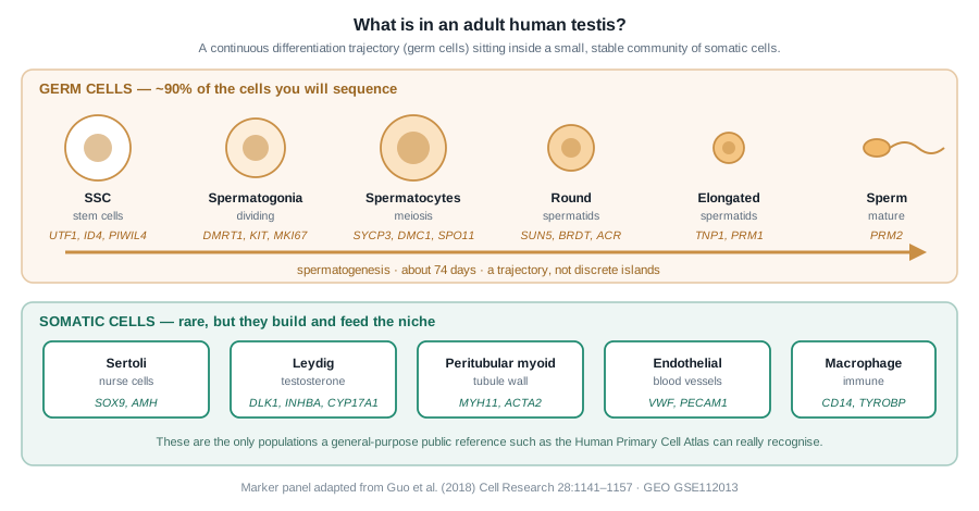
We will use the adult human testis atlas of Guo et al. (2018), GEO accession GSE112013: 6,490 cells from three healthy young donors, two 10x Genomics runs each.

It is a nice teaching dataset because it contains two very different kinds of biology at once, and you will see both on the same UMAP:

Cell types of the adult human testis

---

Step 1: refresher — SummarizedExperiment

This is the container you already met. A rectangle of numbers, plus metadata on its rows, plus metadata on its columns, locked together so they can never fall out of sync.

library(airway)
library(SummarizedExperiment)

data(airway)
se <- airway
se
#> class: RangedSummarizedExperiment 
#> dim: 63677 8 
#> metadata(1): ''
#> assays(1): counts
#> rownames(63677): ENSG00000000003 ENSG00000000005 ... ENSG00000273492
#>   ENSG00000273493
#> rowData names(10): gene_id gene_name ... seq_coord_system symbol
#> colnames(8): SRR1039508 SRR1039509 ... SRR1039520 SRR1039521
#> colData names(9): SampleName cell ... Sample BioSample

Read that printout carefully — it is the map of the object:

dim(se)                    # genes x samples
#> [1] 63677     8
assayNames(se)             # the matrices inside
#> [1] "counts"
head(assay(se, "counts")[, 1:4])
#>                 SRR1039508 SRR1039509 SRR1039512 SRR1039513
#> ENSG00000000003        679        448        873        408
#> ENSG00000000005          0          0          0          0
#> ENSG00000000419        467        515        621        365
#> ENSG00000000457        260        211        263        164
#> ENSG00000000460         60         55         40         35
#> ENSG00000000938          0          0          2          0

Column metadata: one row per sample.

colData(se)[, c("cell", "dex")]
#> DataFrame with 8 rows and 2 columns
#>                cell      dex
#>            <factor> <factor>
#> SRR1039508  N61311     untrt
#> SRR1039509  N61311     trt  
#> SRR1039512  N052611    untrt
#> SRR1039513  N052611    trt  
#> SRR1039516  N080611    untrt
#> SRR1039517  N080611    trt  
#> SRR1039520  N061011    untrt
#> SRR1039521  N061011    trt

Row metadata: one row per gene.

head(rowData(se), 3)
#> DataFrame with 3 rows and 10 columns
#>                         gene_id   gene_name  entrezid   gene_biotype
#>                     <character> <character> <integer>    <character>
#> ENSG00000000003 ENSG00000000003      TSPAN6        NA protein_coding
#> ENSG00000000005 ENSG00000000005        TNMD        NA protein_coding
#> ENSG00000000419 ENSG00000000419        DPM1        NA protein_coding
#>                 gene_seq_start gene_seq_end    seq_name seq_strand
#>                      <integer>    <integer> <character>  <integer>
#> ENSG00000000003       99883667     99894988           X         -1
#> ENSG00000000005       99839799     99854882           X          1
#> ENSG00000000419       49551404     49575092          20         -1
#>                 seq_coord_system      symbol
#>                        <integer> <character>
#> ENSG00000000003               NA      TSPAN6
#> ENSG00000000005               NA        TNMD
#> ENSG00000000419               NA        DPM1

And the two operations you will use constantly. $ reaches into colData():

table(se$dex, se$cell)
#>        
#>         N052611 N061011 N080611 N61311
#>   trt         1       1       1      1
#>   untrt       1       1       1      1

…and [ subsets rows and columns together, keeping everything consistent:

expressed <- rowSums(assay(se, "counts")) > 0
treated <- se[expressed, se$dex == "trt"]
dim(treated)
#> [1] 33469     4
colData(treated)$dex
#> [1] trt trt trt trt
#> Levels: trt untrt

That is the whole idea. A SingleCellExperiment is a SummarizedExperiment with a few extra slots — you already know 80% of the API.

---

Step 2: refresher — DESeq2 in a dozen lines

We are not going to use DESeq2 for most of the workshop, but it is worth having the bulk workflow fresh in your mind, because in Session 2 we will repeatedly ask “why can I not just do that here?”.

Eight samples, four cell lines, treated or untreated with a drug:

library(DESeq2)

se$dex <- relevel(se$dex, ref = "untrt")   # make "untrt" the baseline
levels(se$dex)
#> [1] "untrt" "trt"

Build the model object. The design formula says “account for the cell line, then test the treatment”:

dds <- DESeqDataSet(se, design = ~ cell + dex)

keep <- rowSums(counts(dds) >= 10) >= 4     # drop genes seen in very few samples
dds <- dds[keep, ]
dim(dds)
#> [1] 16139     8

Fit and extract:

dds <- DESeq(dds)
res <- results(dds, contrast = c("dex", "trt", "untrt"))
summary(res)
#> 
#> out of 16139 with nonzero total read count
#> adjusted p-value < 0.1
#> LFC > 0 (up)       : 2607, 16%
#> LFC < 0 (down)     : 2298, 14%
#> outliers [1]       : 0, 0%
#> low counts [2]     : 626, 3.9%
#> (mean count < 12)
#> [1] see 'cooksCutoff' argument of ?results
#> [2] see 'independentFiltering' argument of ?results

head(res[order(res$padj), c("baseMean", "log2FoldChange", "padj")])
#> log2 fold change (MLE): dex trt vs untrt 
#>  
#> DataFrame with 6 rows and 3 columns
#>                  baseMean log2FoldChange         padj
#>                 <numeric>      <numeric>    <numeric>
#> ENSG00000152583   997.961        4.57094 5.53013e-132
#> ENSG00000165995   495.567        3.28708 5.53013e-132
#> ENSG00000120129  3411.966        2.94386 1.24857e-124
#> ENSG00000101347 12712.946        3.76302 2.90930e-124
#> ENSG00000189221  2343.573        3.34972 3.53804e-119
#> ENSG00000211445 12298.197        3.72641 1.34490e-106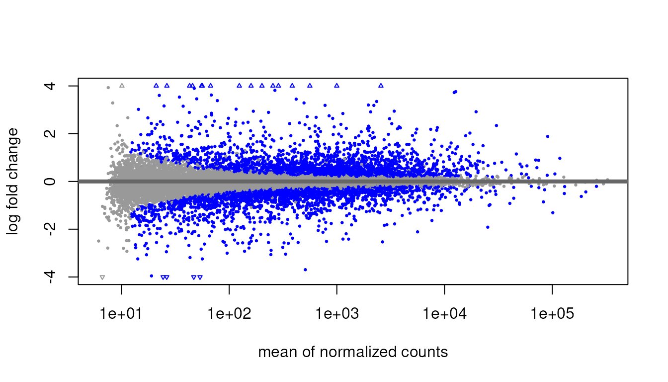

plotMA(res, ylim = c(-4, 4))

Three things to carry with you into Session 2:

1. DESeq2 models raw counts with a negative binomial distribution and estimates a dispersion per gene. It never wants normalised or logged input.
2. The replicates are biological samples, not measurements. Eight columns here means eight independent biological units, which is what makes the p-values mean something.
3. The design formula is where the experiment lives. ~ cell + dex is a statement about how the data were generated.

---

Step 3: what changes when the columns become cells

	Bulk RNA-seq	Single-cell RNA-seq
A column is	a biological sample	one cell
Columns	3–100	2,000–2,000,000
Zeros	few	90–95% of the matrix
Library size varies by	prep efficiency	prep efficiency and cell size, cell state
Groups are	known from the design	discovered by clustering
Replication	built into the design	one donor can give 10,000 cells and still be n = 1
Container	SummarizedExperiment	SingleCellExperiment
Typical DE tool	DESeq2, edgeR, limma	scran for markers; DESeq2 on pseudobulk across samples

The last two rows are the ones that catch people out, and we will come back to them in Session 2.

---

Where to read more

• Orchestrating Single-Cell Analysis with Bioconductor (OSCA) — the reference text for everything in this workshop. Start with OSCA: Introduction.
• The SingleCellExperiment vignette
• Guo J, Grow EJ, Mlcochova H, et al. (2018). The adult human testis transcriptional cell atlas. Cell Research 28:1141–1157.

Next: Session 1 — from a count matrix to a map of the cells.

sessionInfo()
#> R version 4.6.0 (2026-04-24)
#> Platform: x86_64-pc-linux-gnu
#> Running under: Ubuntu 24.04.4 LTS
#> 
#> Matrix products: default
#> BLAS:   /usr/lib/x86_64-linux-gnu/openblas-pthread/libblas.so.3 
#> LAPACK: /usr/lib/x86_64-linux-gnu/openblas-pthread/libopenblasp-r0.3.26.so;  LAPACK version 3.12.0
#> 
#> locale:
#>  [1] LC_CTYPE=en_US.UTF-8       LC_NUMERIC=C              
#>  [3] LC_TIME=en_US.UTF-8        LC_COLLATE=en_US.UTF-8    
#>  [5] LC_MONETARY=en_US.UTF-8    LC_MESSAGES=en_US.UTF-8   
#>  [7] LC_PAPER=en_US.UTF-8       LC_NAME=C                 
#>  [9] LC_ADDRESS=C               LC_TELEPHONE=C            
#> [11] LC_MEASUREMENT=en_US.UTF-8 LC_IDENTIFICATION=C       
#> 
#> time zone: Etc/UTC
#> tzcode source: system (glibc)
#> 
#> attached base packages:
#> [1] stats4    stats     graphics  grDevices utils     datasets  methods  
#> [8] base     
#> 
#> other attached packages:
#>  [1] DESeq2_1.53.2               airway_1.33.2              
#>  [3] SummarizedExperiment_1.43.0 Biobase_2.73.2             
#>  [5] GenomicRanges_1.65.1        Seqinfo_1.3.2              
#>  [7] IRanges_2.47.5              S4Vectors_0.51.9           
#>  [9] BiocGenerics_0.59.12        generics_0.1.4             
#> [11] MatrixGenerics_1.25.0       matrixStats_1.5.0          
#> 
#> loaded via a namespace (and not attached):
#>  [1] sass_0.4.10         SparseArray_1.13.2  lattice_0.23-1     
#>  [4] magrittr_2.0.5      digest_0.6.39       RColorBrewer_1.1-3 
#>  [7] evaluate_1.0.5      grid_4.6.0          fastmap_1.2.0      
#> [10] jsonlite_2.0.0      Matrix_1.7-6        scales_1.4.0       
#> [13] codetools_0.2-20    textshaping_1.0.5   jquerylib_0.1.4    
#> [16] abind_1.4-8         cli_3.6.6           rlang_1.3.0        
#> [19] XVector_0.53.0      cachem_1.1.0        DelayedArray_0.39.6
#> [22] yaml_2.3.12         otel_0.2.0          S4Arrays_1.13.0    
#> [25] tools_4.6.0         parallel_4.6.0      BiocParallel_1.47.0
#> [28] dplyr_1.2.1         ggplot2_4.0.3       locfit_1.5-9.12    
#> [31] vctrs_0.7.3         R6_2.6.1            lifecycle_1.0.5    
#> [34] fs_2.1.0            htmlwidgets_1.6.4   ragg_1.5.2         
#> [37] pkgconfig_2.0.3     desc_1.4.3          pillar_1.11.1      
#> [40] pkgdown_2.2.1       bslib_0.12.0        gtable_0.3.6       
#> [43] glue_1.8.1          Rcpp_1.1.2          systemfonts_1.3.2  
#> [46] tidyselect_1.2.1    tibble_3.3.1        xfun_0.60          
#> [49] knitr_1.51          farver_2.1.2        htmltools_0.5.9    
#> [52] rmarkdown_2.32      compiler_4.6.0      S7_0.2.2