Session 1: from a count matrix to a map of the cells
Jacques Serizay
2026-09-02
Source:vignettes/b_session1.Rmd
b_session1.RmdGoals of this session
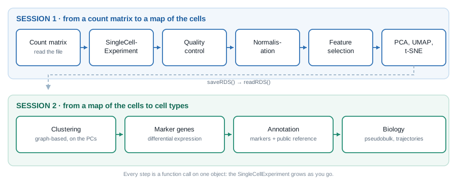
| # | Step | Time |
|---|---|---|
| 1 | What a single-cell count matrix is | 5 min |
| 2 | Reading it into R | 8 min |
| 3 | Building a SingleCellExperiment
|
8 min |
| 4 | Quality control | 14 min |
| 5 | Normalisation | 8 min |
| 6 | Feature selection | 6 min |
| 7 | Dimensionality reduction | 10 min |
| 8 | Saving the object | 2 min |
Every step below adds something to one object. By
the end of the hour, sce will carry the counts, the
normalised values, the cell metadata, the gene statistics and two 2-D
embeddings — and Session 2 starts from exactly that.
1. What is a single-cell count matrix?
We are not going to talk about how it is produced — no droplets, no barcodes, no alignment. Assume someone handed you the file. What is in it?
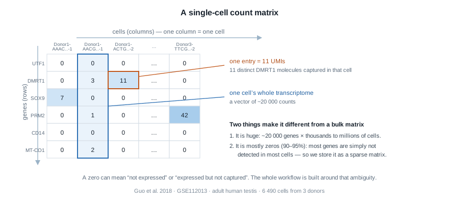
Three ideas to hold on to:
- A column is one cell. Its ~20,000 numbers are that cell’s transcriptome.
- An entry is a UMI count: the number of distinct molecules of that gene captured in that cell. Not reads — molecules. That is why the numbers are small.
- Most entries are zero, and a zero is ambiguous: the gene may be off, or it may be on but missed by a technique that only captures a small fraction of the RNA in a cell. Almost every design decision downstream exists because of that ambiguity.
2. Reading it into R
Importing data from a local count matrix file
The file is already on your disk, cached by
BiocFileCache. Asking for it again costs nothing:
library(BiocFileCache)
bfc <- BiocFileCache(ask = FALSE)
umi_url <- "https://ftp.ncbi.nlm.nih.gov/geo/series/GSE112nnn/GSE112013/suppl/GSE112013_Combined_UMI_table.txt.gz"
umi_path <- bfcrpath(bfc, umi_url)
Let’s import the data using read.delim()
umi <- read.delim(umi_path, header = TRUE, row.names = 1)
dim(umi)
#> [1] 27477  6490
umi[1:5, 1:4]
#>              Donor2.AAACCTGGTGCCTTGG.1 Donor2.AAACCTGTCAACGGGA.1
#> RP11-34P13.3                         0                         0
#> RP11-34P13.7                         0                         0
#> FO538757.3                           0                         0
#> FO538757.2                           0                         1
#> AP006222.2                           0                         0
#>              Donor2.AAACCTGTCCTATGTT.1 Donor2.AAACCTGTCGGACAAG.1
#> RP11-34P13.3                         0                         0
#> RP11-34P13.7                         0                         0
#> FO538757.3                           0                         0
#> FO538757.2                           0                         0
#> AP006222.2                           0                         0
A data.frame is not a matrix: fix that, and get a real
matrix:
genes <- rownames(umi)
counts_dense <- as.matrix(umi)
rownames(counts_dense) <- genes

dim(counts_dense)
#> [1] 27477  6490
counts_dense[1:4, 1:3]
#>              Donor2.AAACCTGGTGCCTTGG.1 Donor2.AAACCTGTCAACGGGA.1
#> RP11-34P13.3                         0                         0
#> RP11-34P13.7                         0                         0
#> FO538757.3                           0                         0
#> FO538757.2                           0                         1
#>              Donor2.AAACCTGTCCTATGTT.1
#> RP11-34P13.3                         0
#> RP11-34P13.7                         0
#> FO538757.3                           0
#> FO538757.2                           0
Make it sparse
Right now the matrix stores every single zero explicitly. Let us see what that costs, and what we save by switching to a sparse representation:
library(Matrix)
counts_sparse <- Matrix(counts_dense, sparse = TRUE)
class(counts_sparse)
#> [1] "dgCMatrix"
#> attr(,"package")
#> [1] "Matrix"
How empty is it really?
We no longer need the dense copy. Free the memory explicitly — with objects this size it matters:
3. Building a SingleCellExperiment
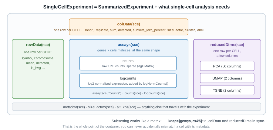
A SingleCellExperiment is a
SummarizedExperiment: everything you learned about
assay(), rowData(), colData() and
[ still applies. A SingleCellExperiment has
extra slots for the things single-cell analysis needs, for example:
-
reducedDims()for embeddings, -
sizeFactors()for normalisation, -
altExps()for spike-ins or other modalities.
library(SingleCellExperiment)
sce <- SingleCellExperiment(assays = list(counts = counts_sparse))
sce
#> class: SingleCellExperiment
#> dim: 27477 6490
#> metadata(0):
#> assays(1): counts
#> rownames(27477): RP11-34P13.3 RP11-34P13.7 ... AC136612.1 AC145212.4
#> rowData names(0):
#> colnames(6490): Donor2.AAACCTGGTGCCTTGG.1 Donor2.AAACCTGTCAACGGGA.1 ...
#>   Donor1.TTTGTCAGTGTGCGTC.2 Donor1.TTTGTCATCCAAACTG.2
#> colData names(0):
#> reducedDimNames(0):
#> mainExpName: NULL
#> altExpNames(0):
colData(sce) ## empty for now
#> DataFrame with 6490 rows and 0 columns
Cell metadata is hiding in the column names
We have no sample sheet — but the cell names carry the design:
head(colnames(sce), 3)
#> [1] "Donor2.AAACCTGGTGCCTTGG.1" "Donor2.AAACCTGTCAACGGGA.1"
#> [3] "Donor2.AAACCTGTCCTATGTT.1"Donor<N>-<barcode>-<replicate>. Split
it apart and store it where it belongs, in colData():
split_names <- strsplit(colnames(sce), "\\.")
sce$Donor     <- split_names |> purrr::map_chr(1)
sce$Barcode   <- split_names |> purrr::map_chr(2)
sce$Replicate <- split_names |> purrr::map_chr(3)
sce$Sample    <- paste(sce$Donor, sce$Replicate, sep = "_rep")

colData(sce)
#> DataFrame with 6490 rows and 4 columns
#>                                 Donor          Barcode   Replicate      Sample
#>                           <character>      <character> <character> <character>
#> Donor2.AAACCTGGTGCCTTGG.1      Donor2 AAACCTGGTGCCTTGG           1 Donor2_rep1
#> Donor2.AAACCTGTCAACGGGA.1      Donor2 AAACCTGTCAACGGGA           1 Donor2_rep1
#> Donor2.AAACCTGTCCTATGTT.1      Donor2 AAACCTGTCCTATGTT           1 Donor2_rep1
#> Donor2.AAACCTGTCGGACAAG.1      Donor2 AAACCTGTCGGACAAG           1 Donor2_rep1
#> Donor2.AAACGGGAGCTATGCT.1      Donor2 AAACGGGAGCTATGCT           1 Donor2_rep1
#> ...                               ...              ...         ...         ...
#> Donor1.TTTGTCAAGAACTCGG.2      Donor1 TTTGTCAAGAACTCGG           2 Donor1_rep2
#> Donor1.TTTGTCAAGGATGGTC.2      Donor1 TTTGTCAAGGATGGTC           2 Donor1_rep2
#> Donor1.TTTGTCAGTAAGGGAA.2      Donor1 TTTGTCAGTAAGGGAA           2 Donor1_rep2
#> Donor1.TTTGTCAGTGTGCGTC.2      Donor1 TTTGTCAGTGTGCGTC           2 Donor1_rep2
#> Donor1.TTTGTCATCCAAACTG.2      Donor1 TTTGTCATCCAAACTG           2 Donor1_rep2
table(sce$Donor, sce$Replicate)
#>
#>             1    2
#>   Donor1 1000 1248
#>   Donor2  985 1009
#>   Donor3 1116 1132
Three donors, two 10x runs each: six samples. Remember that number — in Session 2 it is the difference between a real statistical test and a fake one.
4. Quality control
Not every column of the matrix is a healthy cell. Some are empty droplets that caught ambient RNA, some are cells that were dying when they were captured, some are two cells stuck together. We remove them before anything else, because they distort normalisation, feature selection and clustering.
The three classic signals:
| Signal | Low-quality cells show | Because |
|---|---|---|
Library size (sum) |
very low | little RNA captured |
Genes detected (detected) |
very low | idem |
| Mitochondrial fraction | very high | the cell membrane broke and cytoplasmic mRNA leaked out; mitochondrial transcripts stayed behind |
Compute QC metrics
Mitochondrial genes are recognisable by their symbol:
mito <- grep("^MT-", rownames(sce), value = TRUE)
length(mito)
#> [1] 13
head(mito)
#> [1] "MT-ND1"  "MT-ND2"  "MT-CO1"  "MT-CO2"  "MT-ATP8" "MT-ATP6"
quickRnaQc.se() computes everything in one pass and
writes it straight into colData(). It also suggests QC
thresholds based on the data, by calling a cell an outlier if it sits
more than 3 median absolute deviations from the median of the dataset,
on the log scale.
Because our six samples may have been sequenced to different depths,
we compute the thresholds within each sample using
block.
library(scrapper)
sce <- quickRnaQc.se(sce, subsets = list(Mito = mito), block = sce$Sample)
colData(sce)
#> DataFrame with 6490 rows and 8 columns
#>                                 Donor          Barcode   Replicate      Sample
#>                           <character>      <character> <character> <character>
#> Donor2.AAACCTGGTGCCTTGG.1      Donor2 AAACCTGGTGCCTTGG           1 Donor2_rep1
#> Donor2.AAACCTGTCAACGGGA.1      Donor2 AAACCTGTCAACGGGA           1 Donor2_rep1
#> Donor2.AAACCTGTCCTATGTT.1      Donor2 AAACCTGTCCTATGTT           1 Donor2_rep1
#> Donor2.AAACCTGTCGGACAAG.1      Donor2 AAACCTGTCGGACAAG           1 Donor2_rep1
#> Donor2.AAACGGGAGCTATGCT.1      Donor2 AAACGGGAGCTATGCT           1 Donor2_rep1
#> ...                               ...              ...         ...         ...
#> Donor1.TTTGTCAAGAACTCGG.2      Donor1 TTTGTCAAGAACTCGG           2 Donor1_rep2
#> Donor1.TTTGTCAAGGATGGTC.2      Donor1 TTTGTCAAGGATGGTC           2 Donor1_rep2
#> Donor1.TTTGTCAGTAAGGGAA.2      Donor1 TTTGTCAGTAAGGGAA           2 Donor1_rep2
#> Donor1.TTTGTCAGTGTGCGTC.2      Donor1 TTTGTCAGTGTGCGTC           2 Donor1_rep2
#> Donor1.TTTGTCATCCAAACTG.2      Donor1 TTTGTCATCCAAACTG           2 Donor1_rep2
#>                                 sum  detected subset.proportion.Mito      keep
#>                           <numeric> <integer>              <numeric> <logical>
#> Donor2.AAACCTGGTGCCTTGG.1     11454      4323             0.00934171      TRUE
#> Donor2.AAACCTGTCAACGGGA.1     10149      1613             0.00413834      TRUE
#> Donor2.AAACCTGTCCTATGTT.1     11672      2212             0.01070939      TRUE
#> Donor2.AAACCTGTCGGACAAG.1      9140      1884             0.01039387      TRUE
#> Donor2.AAACGGGAGCTATGCT.1      7849      1991             0.00394955      TRUE
#> ...                             ...       ...                    ...       ...
#> Donor1.TTTGTCAAGAACTCGG.2      5648      2730             0.16643059      TRUE
#> Donor1.TTTGTCAAGGATGGTC.2      5942      3098             0.01565130      TRUE
#> Donor1.TTTGTCAGTAAGGGAA.2     59903      7522             0.04675893      TRUE
#> Donor1.TTTGTCAGTGTGCGTC.2      6499      1720             0.04754578      TRUE
#> Donor1.TTTGTCATCCAAACTG.2      5910      3109             0.00896785      TRUE
summary(sce$sum)
#>    Min. 1st Qu.  Median    Mean 3rd Qu.    Max.
#>    2826    5892    8487   12341   14332  150004
summary(sce$detected)
#>    Min. 1st Qu.  Median    Mean 3rd Qu.    Max.
#>     679    1767    2572    3082    3966    9838
summary(sce$subsets_Mito_percent)
#> Length  Class   Mode
#>      0   NULL   NULL
summary(sce$keep)
#>    Mode   FALSE    TRUE
#> logical     907    5583
Look before you filter
Always plot what you are about to throw away!
library(scater)
library(ggplot2)

plotColData(sce, x = "sum", y = "detected", colour_by = "Sample") +
    scale_x_log10() +
    scale_y_log10() +
    facet_grid(~sce$keep)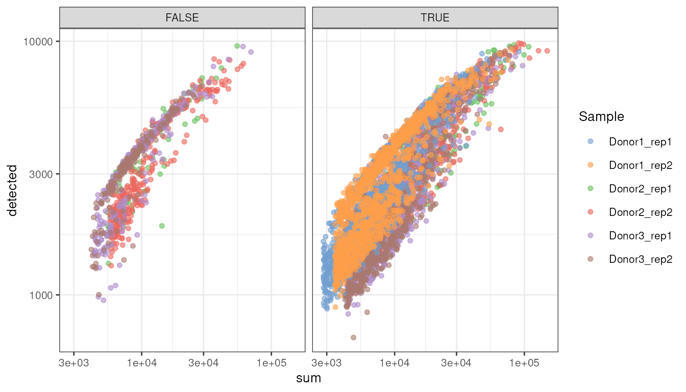
plotColData(sce, x = "detected", y = "subset.proportion.Mito", colour_by = "Sample") +
    scale_x_log10() +
    facet_grid(~sce$keep)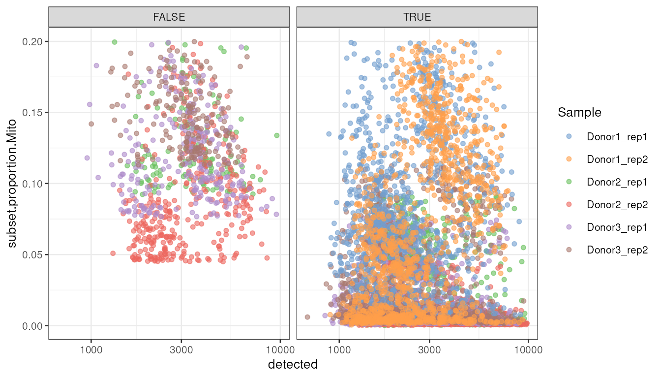
sce <- sce[, sce$keep]
dim(sce)
#> [1] 27477  5583
5. Normalisation
Two cells can differ in total counts for two reasons: one is bigger or more transcriptionally active (biology), or one was captured more efficiently (technology). Normalisation tries to remove the second.
The naive fix is to divide each cell by its library size. That fails when different cell types express very different numbers of genes — exactly our situation, since sperm are transcriptionally almost silent while spermatocytes are not.
scran’s deconvolution method pools
similar cells together to get stable estimates, then deconvolves them
back to individual cells:
library(scran)

set.seed(2026)
clust <- quickCluster(sce)
table(clust)
#> clust
#>   1   2   3   4   5   6   7   8   9  10  11  12  13  14  15  16
#> 416 249 282 334 708 697 596 389 448 335 191 197 111 224 235 171
sce <- computeSumFactors(sce, clusters = clust)
sce$sf <- sizeFactors(sce)
summary(sce$sf)
#>     Min.  1st Qu.   Median     Mean  3rd Qu.     Max.
#>  0.05869  0.25489  0.50735  1.00000  1.16406 15.89853
plotColData(sce, x = "sum", y = "sf", colour_by = "Sample") +
    scale_x_log10() +
    scale_y_log10()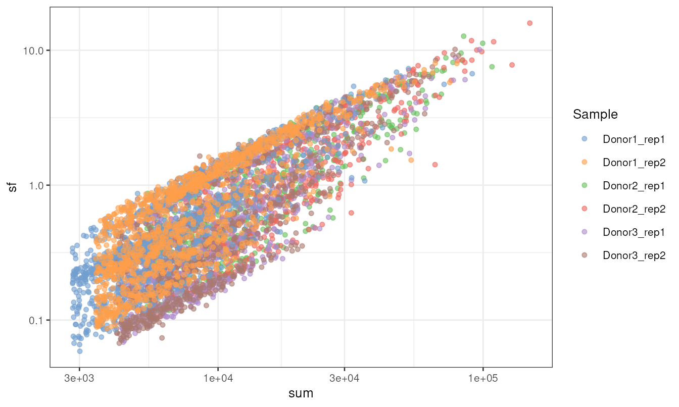
If size factors were just library sizes, this would be a perfect straight line. The spread away from the diagonal is composition bias — the thing we are correcting.
Now apply them and log-transform:
sce <- logNormCounts(sce)
assayNames(sce)
#> [1] "counts"    "logcounts"
logcounts(sce)[1:4, 1:3]
#> 4 x 3 sparse Matrix of class "dgCMatrix"
#>              Donor2.AAACCTGGTGCCTTGG.1 Donor2.AAACCTGTCAACGGGA.1
#> RP11-34P13.3                         .                  .
#> RP11-34P13.7                         .                  .
#> FO538757.3                           .                  .
#> FO538757.2                           .                  2.683887
#>              Donor2.AAACCTGTCCTATGTT.1
#> RP11-34P13.3                         .
#> RP11-34P13.7                         .
#> FO538757.3                           .
#> FO538757.2                           .
logNormCounts() divides each count by the cell’s size
factor, adds a pseudo-count of 1, and takes log2. From here
on, everything that is about expression uses
logcounts; everything that is about counts
(differential expression, later) goes back to counts.
6. Feature selection
We have ~27,000 genes but only “variable” genes carry any information about which cell is which. The rest are either off everywhere, or on everywhere. Keeping them adds noise to the distance calculations that clustering depends on.
The trick is for each gene, compare its variance to what you would expect for a gene of that mean expression. Genes above the trend are interesting.
dec <- modelGeneVar(sce)
dec[1:4, 1:4]
#> DataFrame with 4 rows and 4 columns
#>                    mean      total       tech          bio
#>               <numeric>  <numeric>  <numeric>    <numeric>
#> RP11-34P13.3 0.00215469 0.00322462 0.00324962 -2.50068e-05
#> RP11-34P13.7 0.01186605 0.01671651 0.01789048 -1.17397e-03
#> FO538757.3   0.00270630 0.00433274 0.00408146  2.51281e-04
#> FO538757.2   0.38686195 0.52852532 0.58349437 -5.49691e-02
This separates the variance of gene expression into its technical component (the expected variance at each expression level) and its biological component (the variance due to biological differences).
We can then select the most variable genes (HVGs) for downstream analysis, based on this biological component.
hvg <- getTopHVGs(dec, n = 2000)
length(hvg)
#> [1] 2000
head(hvg, 20)
#>  [1] "TNP1"        "AC007557.1"  "MALAT1"      "HMGB4"       "LELP1"
#>  [6] "CRISP2"      "TSACC"       "LINC00467"   "NUPR2"       "PTGDS"
#> [11] "SMCP"        "IGFBP7"      "OAZ3"        "SPTY2D1-AS1" "TMSB4X"
#> [16] "DCUN1D1"     "RPL10"       "GSG1"        "B2M"         "C10orf62"
Recognise anything? TNP1,
SMCP, GSG1, and others are key genes regulated
during spermatogenesis. Feature selection has found the dominant axis of
variation in a testis without being told anything about testes.
If your samples had been processed on different days, you would add
block = sce$Sample here so that the trend is fitted within
each batch.
7. Dimensionality reduction
2,000 genes is still 2,000 dimensions. PCA compresses them to a few dozen components that capture the structure, and, because noise is spread evenly across components while biology is concentrated in the first few, it denoises at the same time.
set.seed(2026)
sce <- runPCA(sce, ncomponents = 50, subset_row = hvg)

reducedDimNames(sce)
#> [1] "PCA"
dim(reducedDim(sce, "PCA"))
#> [1] 5583   50
How many components are worth keeping?
pct <- attr(reducedDim(sce, "PCA"), "percentVar")
qplot(seq_along(pct), pct, geom = "col") +
    xlab("PC") +
    ylab("Variance explained (%)") +
    geom_vline(xintercept = 20, colour = "red", linetype = 2)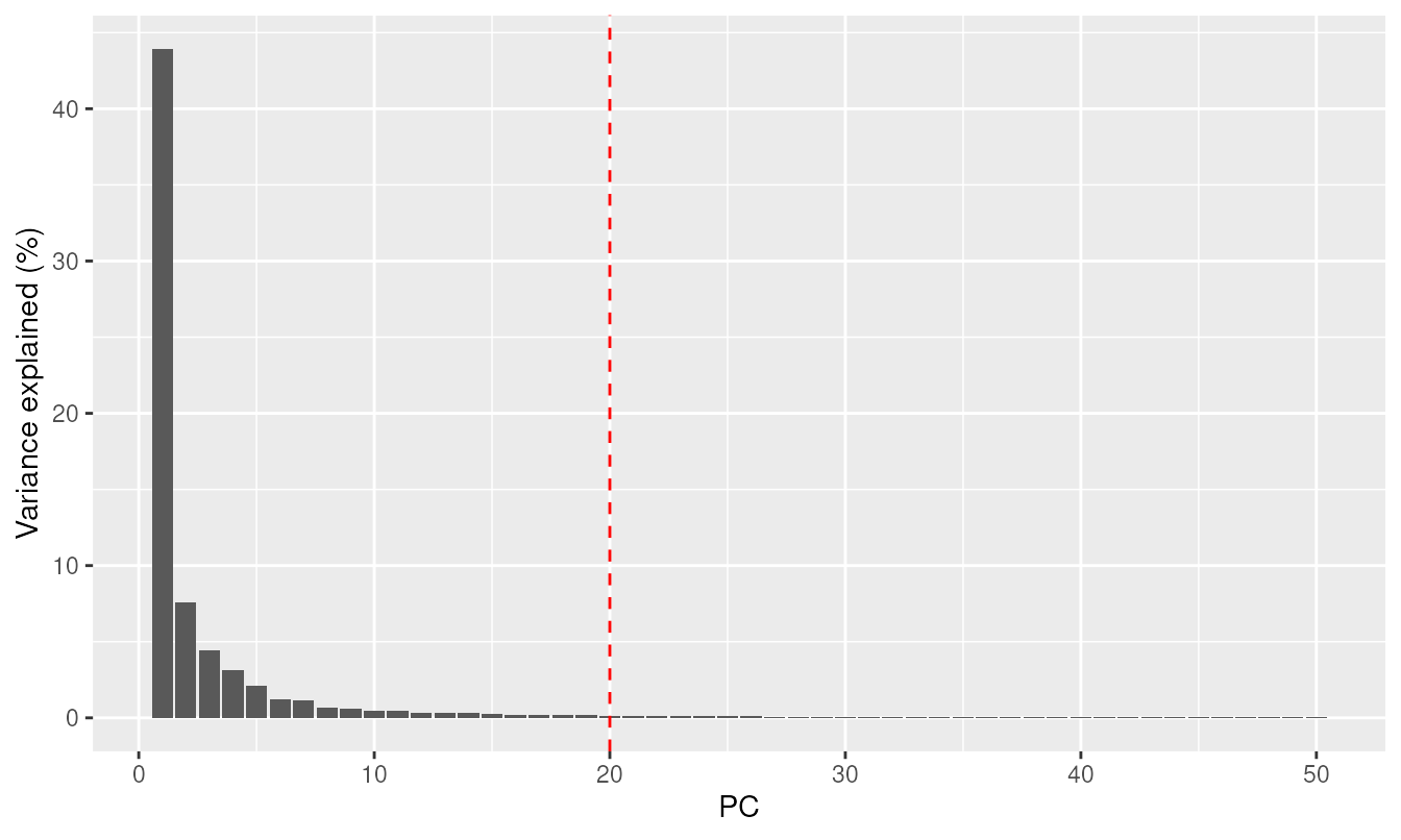
There is no correct answer; the elbow is a guide, and anything between 10 and 30 would give a similar picture here. We will use 20.
plotReducedDim(sce, dimred = "PCA", colour_by = "Donor")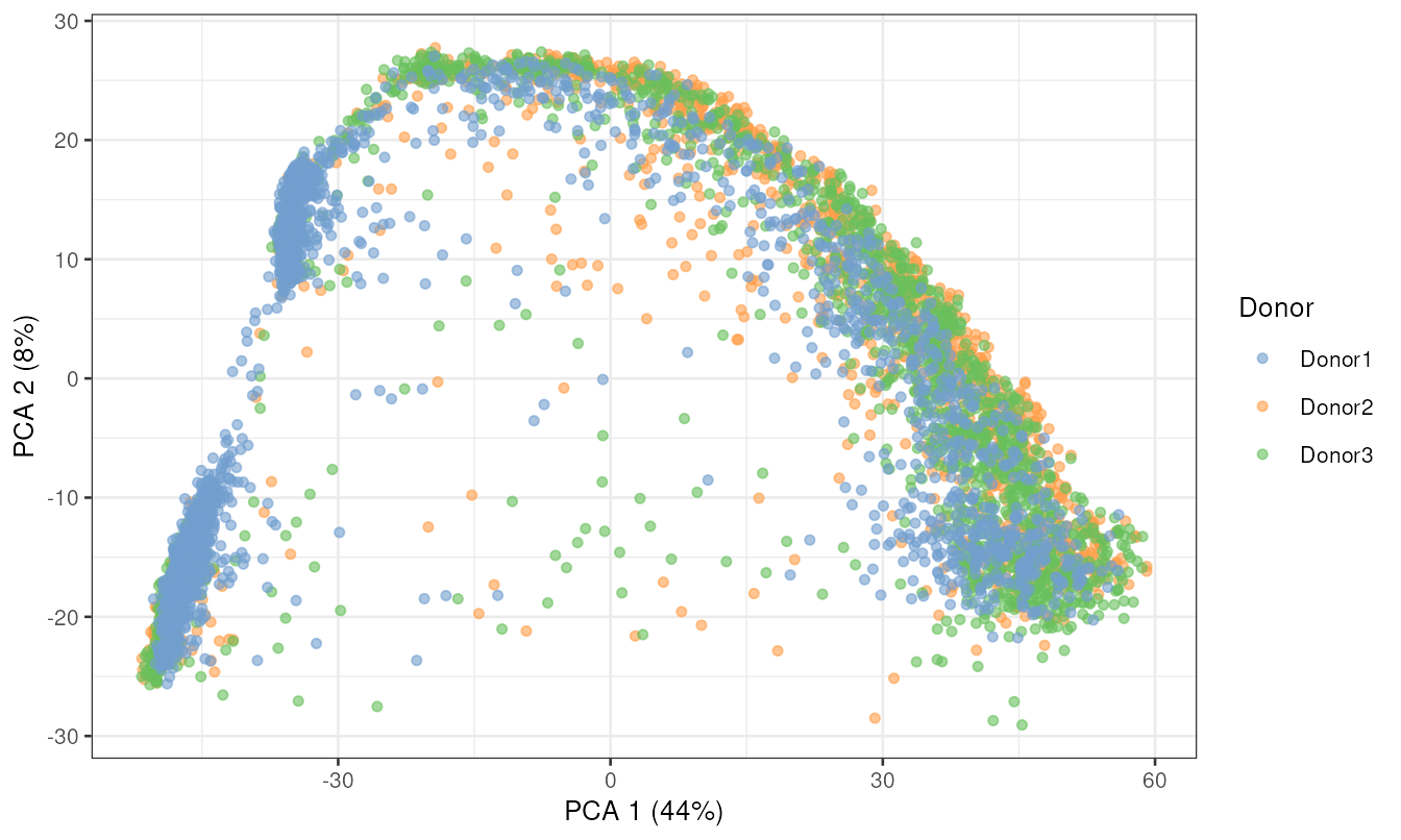
UMAP
PCA is faithful but hard to read. UMAP squeezes the first 20 PCs into two dimensions that we can actually look at:
set.seed(2026)
sce <- runUMAP(sce, dimred = "PCA", n_dimred = 20)
reducedDimNames(sce)
#> [1] "PCA"  "UMAP"
plotUMAP(sce, colour_by = "Donor")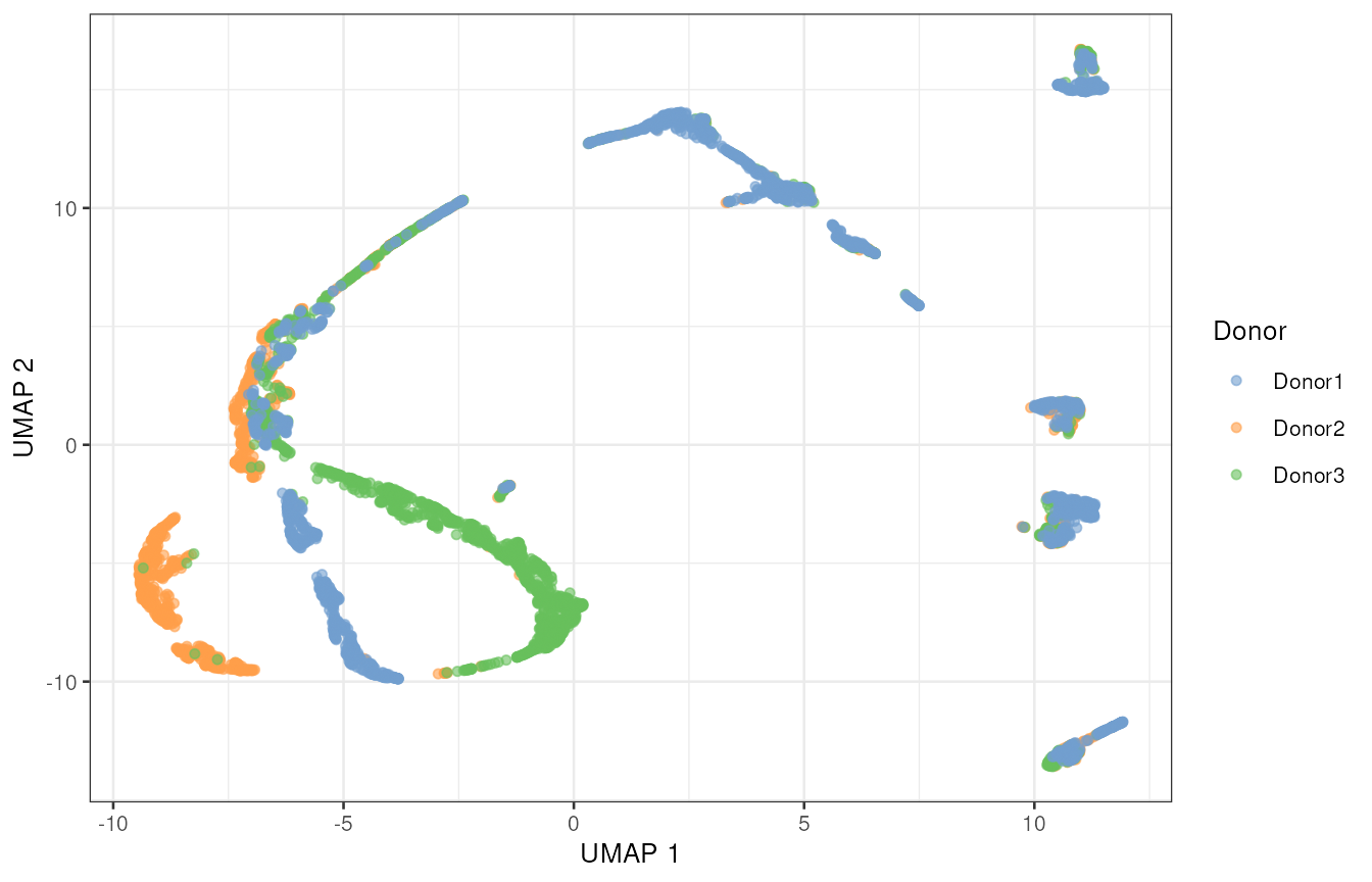
Do the donors overlap, or does each one form its own island? This is the first thing to look at, every time.
- If they overlap, the dominant signal is biological and you can carry on.
- If each donor sits apart, the dominant signal is technical, and you need batch correction before clustering, or you will spend Session 2 annotating donors.
Batch correction
Because distribution of cells across donors is not uniform, we will need to correct for batch effects.
library(batchelor)
set.seed(2026)
corrected_sce <- fastMNN(sce, batch = sce$Donor, d = 20)
corrected_sce
#> class: SingleCellExperiment
#> dim: 27477 5583
#> metadata(2): merge.info pca.info
#> assays(1): reconstructed
#> rownames(27477): RP11-34P13.3 RP11-34P13.7 ... AC136612.1 AC145212.4
#> rowData names(1): rotation
#> colnames(5583): Donor2.AAACCTGGTGCCTTGG.1 Donor2.AAACCTGTCAACGGGA.1 ...
#>   Donor1.TTTGTCAGTGTGCGTC.2 Donor1.TTTGTCATCCAAACTG.2
#> colData names(1): batch
#> reducedDimNames(1): corrected
#> mainExpName: NULL
#> altExpNames(0):

assay(sce, 'reconstructed') <- assay(corrected_sce, 'reconstructed')
reducedDim(sce, 'corrected') <- reducedDim(corrected_sce, 'corrected')
sce <- runUMAP(sce, dimred = "corrected", n_dimred = 20, name = "UMAP_corrected")

plotUMAP(sce, dimred = "UMAP_corrected", colour_by = "Donor")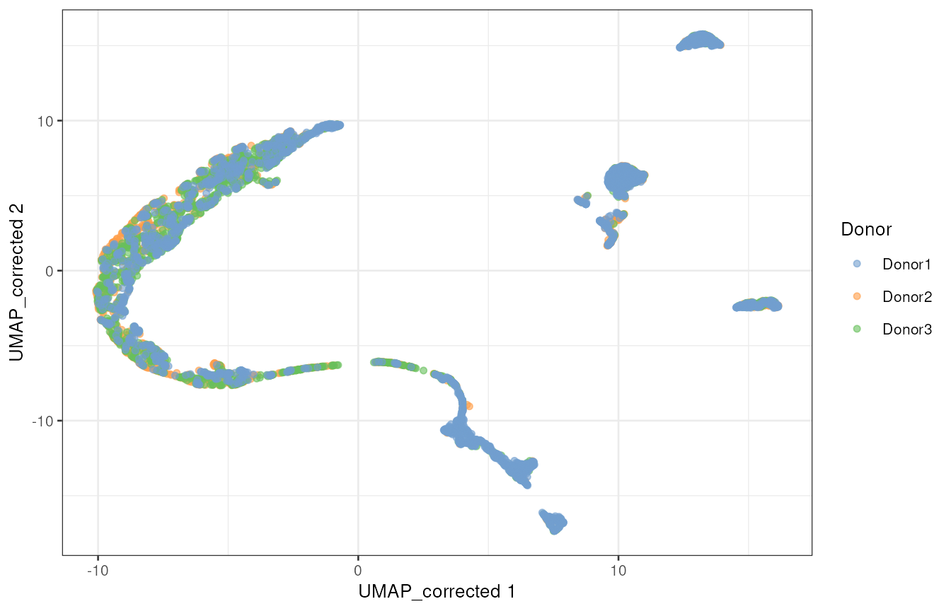
Is any of this real?
Before trusting a picture, check it against something you know. Three genes, three very different territories:
-
UTF1marks the stem cells; -
DMRT1the dividing spermatogonia; -
PRM2the mature spermatids;
library(patchwork)
genes <- c("UTF1", "DMRT1", "PRM2")
wrap_plots(lapply(genes, function(g) {
    plotUMAP(sce, dimred = "UMAP_corrected", colour_by = g) + ggtitle(g)
}), nrow = 2)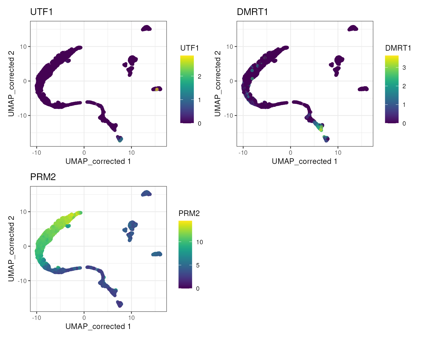
8. Save your object
sce
#> class: SingleCellExperiment
#> dim: 27477 5583
#> metadata(1): qc
#> assays(3): counts logcounts reconstructed
#> rownames(27477): RP11-34P13.3 RP11-34P13.7 ... AC136612.1 AC145212.4
#> rowData names(0):
#> colnames(5583): Donor2.AAACCTGGTGCCTTGG.1 Donor2.AAACCTGTCAACGGGA.1 ...
#>   Donor1.TTTGTCAGTGTGCGTC.2 Donor1.TTTGTCATCCAAACTG.2
#> colData names(10): Donor Barcode ... sizeFactor sf
#> reducedDimNames(4): PCA UMAP corrected UMAP_corrected
#> mainExpName: NULL
#> altExpNames(0):
Look at everything that object now carries: three assays, ten columns of cell metadata, size factors, four reduced dimensions. That is one hour of work in one variable.
Now save it and download it for backup!
saveRDS(sce, "sce_day1.rds")Session 2 begins by reading this file back. If you lose it, there is a catch-up block at the top of the next page that rebuilds it in one go.
Homework
Try these before Session 2. They take about 20 minutes.
1. How many cells did each donor contribute after QC? Which sample lost the largest proportion of its cells, and can you see why in the QC plots?
Hint
table(sce$Sample) after filtering, compared with the same
table before. Then
plotColData(sce, x = "Sample", y = "subsets_Mito_percent").
2. Redo the feature selection with
n = 500 and with n = 5000 HVGs, rerun
runPCA() and runUMAP() for each, and compare
the UMAPs. How sensitive is the picture to that choice?
Hint
Store the results under different names so you can plot them side by side:runPCA(sce, subset_row = hvg500, name = "PCA500"),
then runUMAP(sce, dimred = "PCA500", name = "UMAP500").
3.
plotUMAP(sce, colour_by = "subsets_Mito_percent"). Is there
a region of the map with systematically higher mitochondrial content?
Should you have filtered harder — or is that biology?
4. Use the marker panel from the testis figure to colour the UMAP by
one somatic marker of your choice (VWF, CD14,
ACTA2, DLK1). Where do the somatic cells sit
relative to the germ cells?
What we did
umi             <- read.delim(umi_path, header = TRUE, row.names = 1)     # read
counts_sparse   <- Matrix(as.matrix(umi), sparse = TRUE)              # sparsify
sce             <- SingleCellExperiment(list(counts = counts_sparse))     # build SCE
# build cell metadata
spl_colnames    <- strsplit(colnames(counts_sparse), "\\.")
Donor           <- purrr::map_chr(spl_colnames, 1)
Barcode         <- purrr::map_chr(spl_colnames, 2)
Replicate       <- purrr::map_chr(spl_colnames, 3)
Sample          <- paste(Donor, Replicate, sep = "_rep")
colData(sce)    <- DataFrame(
    Donor = Donor, Barcode = Barcode, Replicate = Replicate, Sample = Sample
)
sce             <- quickRnaQc.se(sce, subsets = list(Mito = mito), block = sce$Sample)  # QC metrics
sce             <- sce[, sce$keep]                                        # filter
sce             <- computeSumFactors(sce, clusters = quickCluster(sce))   # normalise
sce             <- logNormCounts(sce)
dec             <- modelGeneVar(sce); hvg <- getTopHVGs(dec, n = 2000)    # features
sce             <- runPCA(sce, subset_row = hvg, ncomponents = 50)        # reduce
sce             <- runUMAP(sce, dimred = "PCA", n_dimred = 20)            # run UMAP
corrected_sce   <- fastMNN(sce, batch = sce$Donor, d = 20)            # batch correction
reducedDim(sce, "corrected") <- reducedDim(corrected_sce, "corrected")
sce             <- runUMAP(sce, dimred = "corrected", n_dimred = 20, name = "UMAP_corrected") # run UMAP on corrected data
Fourteen function calls. Everything else was looking at the result and deciding whether to believe it — which is the actual job.
Next: Session 2 — from clusters to cell types.
sessionInfo()
#> R version 4.6.0 (2026-04-24)
#> Platform: x86_64-pc-linux-gnu
#> Running under: Ubuntu 24.04.4 LTS
#>
#> Matrix products: default
#> BLAS:   /usr/lib/x86_64-linux-gnu/openblas-pthread/libblas.so.3
#> LAPACK: /usr/lib/x86_64-linux-gnu/openblas-pthread/libopenblasp-r0.3.26.so;  LAPACK version 3.12.0
#>
#> locale:
#>  [1] LC_CTYPE=en_US.UTF-8       LC_NUMERIC=C
#>  [3] LC_TIME=en_US.UTF-8        LC_COLLATE=en_US.UTF-8
#>  [5] LC_MONETARY=en_US.UTF-8    LC_MESSAGES=en_US.UTF-8
#>  [7] LC_PAPER=en_US.UTF-8       LC_NAME=C
#>  [9] LC_ADDRESS=C               LC_TELEPHONE=C
#> [11] LC_MEASUREMENT=en_US.UTF-8 LC_IDENTIFICATION=C
#>
#> time zone: Etc/UTC
#> tzcode source: system (glibc)
#>
#> attached base packages:
#> [1] stats4    stats     graphics  grDevices utils     datasets  methods
#> [8] base
#>
#> other attached packages:
#>  [1] patchwork_1.3.2             batchelor_1.29.0
#>  [3] scran_1.41.1                scater_1.41.2
#>  [5] ggplot2_4.0.3               scuttle_1.23.2
#>  [7] scrapper_1.7.9              SingleCellExperiment_1.35.2
#>  [9] SummarizedExperiment_1.43.0 Biobase_2.73.2
#> [11] GenomicRanges_1.65.1        Seqinfo_1.3.2
#> [13] IRanges_2.47.5              S4Vectors_0.51.9
#> [15] BiocGenerics_0.59.12        generics_0.1.4
#> [17] MatrixGenerics_1.25.0       matrixStats_1.5.0
#> [19] Matrix_1.7-6                BiocFileCache_3.3.0
#> [21] dbplyr_2.6.0
#>
#> loaded via a namespace (and not attached):
#>  [1] DBI_1.3.0                 gridExtra_2.3.1
#>  [3] httr2_1.3.0               rlang_1.3.0
#>  [5] magrittr_2.0.5            RcppAnnoy_0.0.23
#>  [7] otel_0.2.0                compiler_4.6.0
#>  [9] RSQLite_3.53.3            DelayedMatrixStats_1.35.0
#> [11] systemfonts_1.3.2         vctrs_0.7.3
#> [13] pkgconfig_2.0.3           fastmap_1.2.0
#> [15] XVector_0.53.0            labeling_0.4.3
#> [17] rmarkdown_2.32            ggbeeswarm_0.7.3
#> [19] ragg_1.5.2                purrr_1.2.2
#> [21] bit_4.6.0                 xfun_0.60
#> [23] bluster_1.23.1            cachem_1.1.0
#> [25] beachmat_2.29.2           jsonlite_2.0.0
#> [27] blob_1.3.0                DelayedArray_0.39.6
#> [29] BiocParallel_1.47.0       irlba_2.3.7
#> [31] parallel_4.6.0            cluster_2.1.8.3
#> [33] R6_2.6.1                  bslib_0.12.0
#> [35] RColorBrewer_1.1-3        limma_3.99.0
#> [37] jquerylib_0.1.4           Rcpp_1.1.2
#> [39] knitr_1.51                igraph_2.3.3
#> [41] tidyselect_1.2.1          abind_1.4-8
#> [43] yaml_2.3.12               viridis_0.6.5
#> [45] codetools_0.2-20          curl_8.0.0
#> [47] lattice_0.23-1            tibble_3.3.1
#> [49] withr_3.0.3               S7_0.2.2
#> [51] evaluate_1.0.5            desc_1.4.3
#> [53] pillar_1.11.1             filelock_1.0.3
#> [55] sparseMatrixStats_1.25.0  scales_1.4.0
#> [57] glue_1.8.1                metapod_1.21.0
#> [59] tools_4.6.0               BiocNeighbors_2.7.3
#> [61] RSpectra_0.16-2           ScaledMatrix_1.21.0
#> [63] locfit_1.5-9.12           fs_2.1.0
#> [65] grid_4.6.0                edgeR_4.99.1
#> [67] beeswarm_0.4.0            BiocSingular_1.29.1
#> [69] vipor_0.4.7               cli_3.6.6
#> [71] rsvd_1.0.5                textshaping_1.0.5
#> [73] S4Arrays_1.13.0           viridisLite_0.4.3
#> [75] dplyr_1.2.1               ResidualMatrix_1.23.0
#> [77] uwot_0.2.5                gtable_0.3.6
#> [79] sass_0.4.10               digest_0.6.39
#> [81] SparseArray_1.13.2        ggrepel_0.9.8
#> [83] dqrng_0.4.1               htmlwidgets_1.6.4
#> [85] farver_2.1.2              memoise_2.0.1
#> [87] htmltools_0.5.9           pkgdown_2.2.1
#> [89] lifecycle_1.0.5           statmod_1.5.2
#> [91] bit64_4.8.6