library(ggplot2)
library(purrr)
library(GenomicRanges)
##  Loading required package: stats4
##  Loading required package: BiocGenerics
##
##  Attaching package: 'BiocGenerics'
##  The following objects are masked from 'package:stats':
##
##      IQR, mad, sd, var, xtabs
##  The following objects are masked from 'package:base':
##
##      Filter, Find, Map, Position, Reduce, anyDuplicated, aperm,
##      append, as.data.frame, basename, cbind, colnames, dirname,
##      do.call, duplicated, eval, evalq, get, grep, grepl, intersect,
##      is.unsorted, lapply, mapply, match, mget, order, paste, pmax,
##      pmax.int, pmin, pmin.int, rank, rbind, rownames, sapply,
##      setdiff, table, tapply, union, unique, unsplit, which.max,
##      which.min
##  Loading required package: S4Vectors
##
##  Attaching package: 'S4Vectors'
##  The following object is masked from 'package:utils':
##
##      findMatches
##  The following objects are masked from 'package:base':
##
##      I, expand.grid, unname
##  Loading required package: IRanges
##
##  Attaching package: 'IRanges'
##  The following object is masked from 'package:purrr':
##
##      reduce
##  Loading required package: GenomeInfoDb
library(InteractionSet)
##  Loading required package: SummarizedExperiment
##  Loading required package: MatrixGenerics
##  Loading required package: matrixStats
##
##  Attaching package: 'MatrixGenerics'
##  The following objects are masked from 'package:matrixStats':
##
##      colAlls, colAnyNAs, colAnys, colAvgsPerRowSet, colCollapse,
##      colCounts, colCummaxs, colCummins, colCumprods, colCumsums,
##      colDiffs, colIQRDiffs, colIQRs, colLogSumExps, colMadDiffs,
##      colMads, colMaxs, colMeans2, colMedians, colMins, colOrderStats,
##      colProds, colQuantiles, colRanges, colRanks, colSdDiffs, colSds,
##      colSums2, colTabulates, colVarDiffs, colVars, colWeightedMads,
##      colWeightedMeans, colWeightedMedians, colWeightedSds,
##      colWeightedVars, rowAlls, rowAnyNAs, rowAnys, rowAvgsPerColSet,
##      rowCollapse, rowCounts, rowCummaxs, rowCummins, rowCumprods,
##      rowCumsums, rowDiffs, rowIQRDiffs, rowIQRs, rowLogSumExps,
##      rowMadDiffs, rowMads, rowMaxs, rowMeans2, rowMedians, rowMins,
##      rowOrderStats, rowProds, rowQuantiles, rowRanges, rowRanks,
##      rowSdDiffs, rowSds, rowSums2, rowTabulates, rowVarDiffs,
##      rowVars, rowWeightedMads, rowWeightedMeans, rowWeightedMedians,
##      rowWeightedSds, rowWeightedVars
##  Loading required package: Biobase
##  Welcome to Bioconductor
##
##      Vignettes contain introductory material; view with
##      'browseVignettes()'. To cite Bioconductor, see
##      'citation("Biobase")', and for packages 'citation("pkgname")'.
##
##  Attaching package: 'Biobase'
##  The following object is masked from 'package:MatrixGenerics':
##
##      rowMedians
##  The following objects are masked from 'package:matrixStats':
##
##      anyMissing, rowMedians
library(HiCExperiment)
##  Consider using the `HiContacts` package to perform advanced genomic operations
##  on `HiCExperiment` objects.
##
##  Read "Orchestrating Hi-C analysis with Bioconductor" online book to learn more:
##  https://js2264.github.io/OHCA/
##
##  Attaching package: 'HiCExperiment'
##  The following object is masked from 'package:SummarizedExperiment':
##
##      metadata<-
##  The following object is masked from 'package:S4Vectors':
##
##      metadata<-
##  The following object is masked from 'package:ggplot2':
##
##      resolution
library(HiContactsData)
##  Loading required package: ExperimentHub
##  Loading required package: AnnotationHub
##  Loading required package: BiocFileCache
##  Loading required package: dbplyr
##
##  Attaching package: 'AnnotationHub'
##  The following object is masked from 'package:Biobase':
##
##      cache
library(multiHiCcompare)
##
##  Attaching package: 'multiHiCcompare'
##  The following object is masked from 'package:HiCExperiment':
##
##      resolution
##  The following object is masked from 'package:ggplot2':
##
## resolutionWorkflow 3: Inter-centromere interactions in yeast
Pre-loading packages and objects 📦
Aims
This chapter illustrates how to plot the aggregate signal over pairs of genomic ranges, in this case pairs of yeast centromeres.
Datasets
We leverage two yeast datasets in this notebook.
- One from a WT yeast strain in G1 phase
- One from a WT yeast strain in G2/M phase
Importing Hi-C data and plotting contact matrices
library(HiContactsData)
library(HiContacts)
##  Registered S3 methods overwritten by 'readr':
##    method                    from
##    as.data.frame.spec_tbl_df vroom
##    as_tibble.spec_tbl_df     vroom
##    format.col_spec           vroom
##    print.col_spec            vroom
##    print.collector           vroom
##    print.date_names          vroom
##    print.locale              vroom
##    str.col_spec              vroom
library(purrr)
library(ggplot2)
hics <- list(
    'G1' = import(HiContactsData('yeast_g1', 'mcool'), format = 'cool', resolution = 4000),
    'G2M' = import(HiContactsData('yeast_g2m', 'mcool'), format = 'cool', resolution = 4000)
)
##  see ?HiContactsData and browseVignettes('HiContactsData') for documentation
##  downloading 1 resources
##  retrieving 1 resource
##  loading from cache
##  see ?HiContactsData and browseVignettes('HiContactsData') for documentation
##  downloading 1 resources
##  retrieving 1 resource
##  loading from cache
imap(hics, ~ plotMatrix(
    .x, use.scores = 'balanced', limits = c(-4, -1), caption = FALSE
) + ggtitle(.y))
##  $G1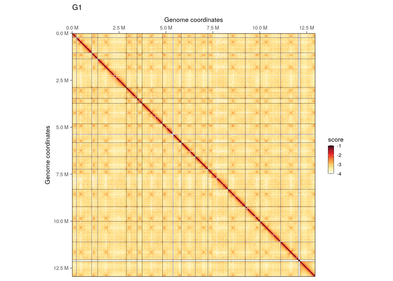
##
##  $G2M
We can visually appreciate that inter-chromosomal interactions, notably between centromeres, are less prominent in G2/M.
Checking P(s) and cis/trans interactions ratio
library(dplyr)
##
##  Attaching package: 'dplyr'
##  The following objects are masked from 'package:dbplyr':
##
##      ident, sql
##  The following object is masked from 'package:Biobase':
##
##      combine
##  The following object is masked from 'package:matrixStats':
##
##      count
##  The following objects are masked from 'package:GenomicRanges':
##
##      intersect, setdiff, union
##  The following object is masked from 'package:GenomeInfoDb':
##
##      intersect
##  The following objects are masked from 'package:IRanges':
##
##      collapse, desc, intersect, setdiff, slice, union
##  The following objects are masked from 'package:S4Vectors':
##
##      first, intersect, rename, setdiff, setequal, union
##  The following objects are masked from 'package:BiocGenerics':
##
##      combine, intersect, setdiff, union
##  The following objects are masked from 'package:stats':
##
##      filter, lag
##  The following objects are masked from 'package:base':
##
##      intersect, setdiff, setequal, union
pairs <- list(
    'G1' = PairsFile(HiContactsData('yeast_g1', 'pairs')),
    'G2M' = PairsFile(HiContactsData('yeast_g2m', 'pairs'))
)
##  see ?HiContactsData and browseVignettes('HiContactsData') for documentation
##  downloading 1 resources
##  retrieving 1 resource
##  loading from cache
##  see ?HiContactsData and browseVignettes('HiContactsData') for documentation
##  downloading 1 resources
##  retrieving 1 resource
##  loading from cache
ps <- imap_dfr(pairs, ~ distanceLaw(.x, by_chr = TRUE) |>
    mutate(sample = .y)
)
##  Importing pairs file /root/.cache/R/ExperimentHub/165c2f428c64_8630 in memory. This may take a while...
##  Importing pairs file /root/.cache/R/ExperimentHub/165c9d9f85c_8631 in memory. This may take a while...
plotPs(ps, aes(x = binned_distance, y = norm_p, group = interaction(sample, chr), color = sample)) +
    scale_color_manual(values = c('black', 'red'))
##  Warning: Removed 2133 rows containing missing values (`geom_line()`).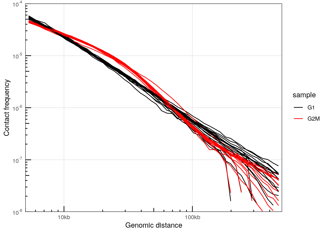
plotPsSlope(ps, ggplot2::aes(x = binned_distance, y = slope, group = interaction(sample, chr), color = sample)) +
    scale_color_manual(values = c('black', 'red'))
##  Warning: Removed 2183 rows containing missing values (`geom_line()`).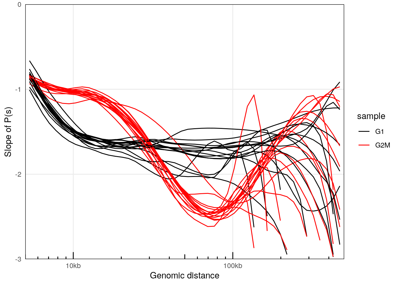
This confirms that interactions in cells synchronized in G2/M are enriched for 10-30kb-long interactions.
ratios <- imap_dfr(hics, ~ cisTransRatio(.x) |> mutate(sample = .y))
ggplot(ratios, aes(x = chr, y = trans_pct, fill = sample)) +
    geom_col() +
    labs(x = 'Chromosomes', y = "% of trans interactions") +
    scale_y_continuous(labels = scales::percent) +
    facet_grid(~sample)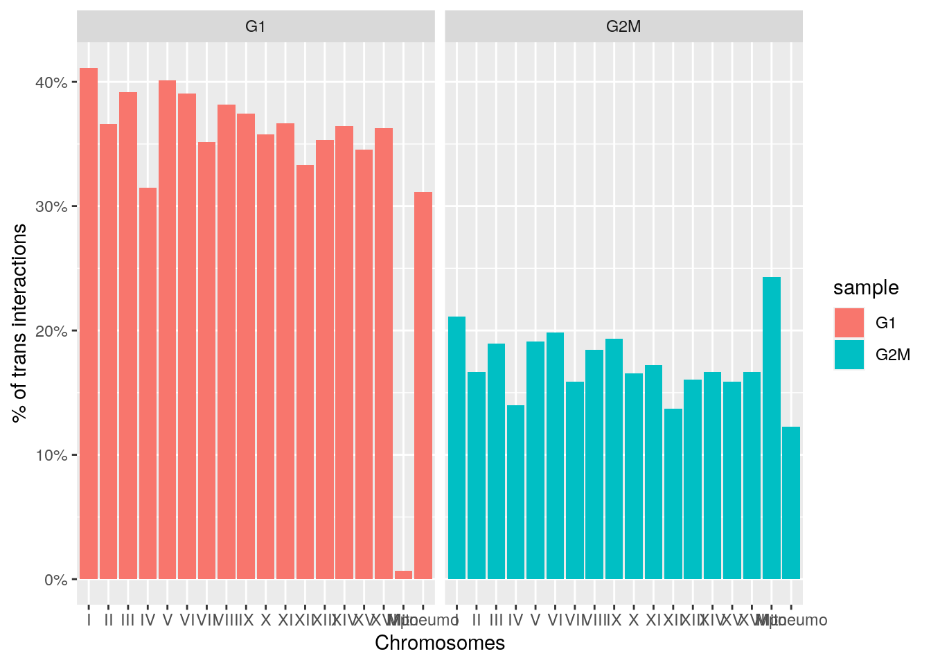
We can also highlight that trans (inter-chromosomal) interactions are proportionally decreasing in G2/M-synchronized cells.
Centromere virtual 4C profiles
data(centros_yeast)
v4c_centro <- imap_dfr(hics, ~ virtual4C(.x, GenomicRanges::resize(centros_yeast[2], 8000)) |>
    as_tibble() |>
    mutate(sample = .y) |>
    filter(seqnames == 'IV')
)
ggplot(v4c_centro, aes(x = start, y = score, fill = sample)) +
    geom_area() +
    theme_bw() +
    labs(
        x = "chrIV position",
        y = "Contacts with chrII centromere",
        title = "Interaction profile of chrII centromere"
    ) +
    coord_cartesian(ylim = c(0, 0.015))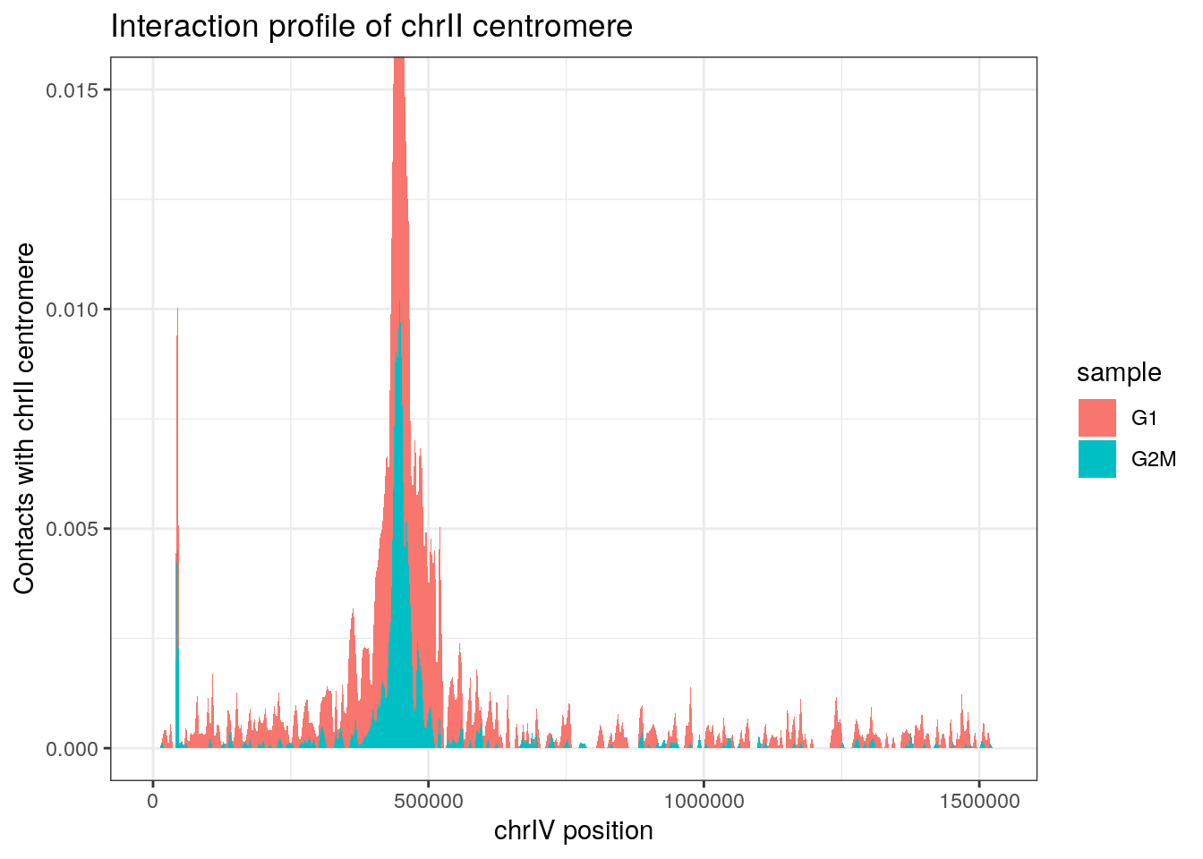
Aggregated 2D signal over all pairs of centromeres
We can start by computing all possible pairs of centromeres.
centros_pairs <- lapply(1:length(centros_yeast), function(i) {
    lapply(1:length(centros_yeast), function(j) {
        S4Vectors::Pairs(centros_yeast[i], centros_yeast[j])
    })
}) |>
    do.call(c, args = _) |>
    do.call(c, args = _) |>
    InteractionSet::makeGInteractionsFromGRangesPairs()
centros_pairs <- centros_pairs[anchors(centros_pairs, 'first') != anchors(centros_pairs, 'second')]

centros_pairs
##  GInteractions object with 240 interactions and 0 metadata columns:
##          seqnames1       ranges1     seqnames2       ranges2
##              <Rle>     <IRanges>         <Rle>     <IRanges>
##      [1]         I 151583-151641 ---        II 238361-238419
##      [2]         I 151583-151641 ---       III 114322-114380
##      [3]         I 151583-151641 ---        IV 449879-449937
##      [4]         I 151583-151641 ---         V 152522-152580
##      [5]         I 151583-151641 ---        VI 147981-148039
##      ...       ...           ... ...       ...           ...
##    [236]       XVI 556255-556313 ---        XI 440229-440287
##    [237]       XVI 556255-556313 ---       XII 151366-151424
##    [238]       XVI 556255-556313 ---      XIII 268222-268280
##    [239]       XVI 556255-556313 ---       XIV 628588-628646
##    [240]       XVI 556255-556313 ---        XV 326897-326955
##    -------
##    regions: 16 ranges and 0 metadata columns
##    seqinfo: 17 sequences (1 circular) from R64-1-1 genome
Then we can aggregate the Hi-C signal over each pair of centromeres.
aggr_maps <- purrr::imap(hics, ~ {
    aggr <- aggregate(.x, centros_pairs, maxDistance = 1e999)
    plotMatrix(
        aggr, use.scores = 'balanced', limits = c(-5, -1),
        cmap = HiContacts::rainbowColors(),
        caption = FALSE
    ) + ggtitle(.y)
})
##  Warning in valid.GenomicRanges.seqinfo(x, suggest.trim = TRUE): GRanges object contains 120 out-of-bound ranges located on sequences
##    I, III, V, VI, VIII, IX, XII, and XIV. Note that ranges located on a
##    sequence whose length is unknown (NA) or on a circular sequence are
##    not considered out-of-bound (use seqlengths() and isCircular() to
##    get the lengths and circularity flags of the underlying sequences).
##    You can use trim() to trim these ranges. See
##    ?`trim,GenomicRanges-method` for more information.
##  Warning in valid.GenomicRanges.seqinfo(x, suggest.trim = TRUE): GRanges object contains 120 out-of-bound ranges located on sequences
##    III, V, VI, VIII, IX, XII, XIV, and I. Note that ranges located on a
##    sequence whose length is unknown (NA) or on a circular sequence are
##    not considered out-of-bound (use seqlengths() and isCircular() to
##    get the lengths and circularity flags of the underlying sequences).
##    You can use trim() to trim these ranges. See
##    ?`trim,GenomicRanges-method` for more information.
##  Warning in valid.GenomicRanges.seqinfo(x, suggest.trim = TRUE): GRanges object contains 240 out-of-bound ranges located on sequences
##    I, III, V, VI, VIII, IX, XII, and XIV. Note that ranges located on a
##    sequence whose length is unknown (NA) or on a circular sequence are
##    not considered out-of-bound (use seqlengths() and isCircular() to
##    get the lengths and circularity flags of the underlying sequences).
##    You can use trim() to trim these ranges. See
##    ?`trim,GenomicRanges-method` for more information.
##  Going through preflight checklist...
##  Parsing the entire contact matrice as a sparse matrix...
##  Modeling distance decay...
##  Filtering for contacts within provided targets...
##  Warning in valid.GenomicRanges.seqinfo(x, suggest.trim = TRUE): GRanges object contains 120 out-of-bound ranges located on sequences
##    I, III, V, VI, VIII, IX, XII, and XIV. Note that ranges located on a
##    sequence whose length is unknown (NA) or on a circular sequence are
##    not considered out-of-bound (use seqlengths() and isCircular() to
##    get the lengths and circularity flags of the underlying sequences).
##    You can use trim() to trim these ranges. See
##    ?`trim,GenomicRanges-method` for more information.
##  Warning in valid.GenomicRanges.seqinfo(x, suggest.trim = TRUE): GRanges object contains 120 out-of-bound ranges located on sequences
##    III, V, VI, VIII, IX, XII, XIV, and I. Note that ranges located on a
##    sequence whose length is unknown (NA) or on a circular sequence are
##    not considered out-of-bound (use seqlengths() and isCircular() to
##    get the lengths and circularity flags of the underlying sequences).
##    You can use trim() to trim these ranges. See
##    ?`trim,GenomicRanges-method` for more information.
##  Warning in valid.GenomicRanges.seqinfo(x, suggest.trim = TRUE): GRanges object contains 240 out-of-bound ranges located on sequences
##    I, III, V, VI, VIII, IX, XII, and XIV. Note that ranges located on a
##    sequence whose length is unknown (NA) or on a circular sequence are
##    not considered out-of-bound (use seqlengths() and isCircular() to
##    get the lengths and circularity flags of the underlying sequences).
##    You can use trim() to trim these ranges. See
##    ?`trim,GenomicRanges-method` for more information.
##  Going through preflight checklist...
##  Parsing the entire contact matrice as a sparse matrix...
##  Modeling distance decay...
##  Filtering for contacts within provided targets...

cowplot::plot_grid(plotlist = aggr_maps, nrow = 1)
Aggregated 1D interaction profile of centromeres
One can generalize the previous virtual 4C plot, by extracting the interaction profile between all possible pairs of centromeres in each dataset.
df <- map_dfr(1:{length(centros_yeast)-1}, function(i) {
    centro1 <- GenomicRanges::resize(centros_yeast[i], fix = 'center', 8000)
    map_dfr({i+1}:length(centros_yeast), function(j) {
        centro2 <- GenomicRanges::resize(centros_yeast[j], fix = 'center', 80000)
        gi <- InteractionSet::GInteractions(centro1, centro2)
        imap_dfr(hics, ~ .x[gi] |>
            interactions() |>
            as_tibble() |>
            mutate(
                sample = .y,
                center = center2 - start(GenomicRanges::resize(centro2, fix = 'center', 1))
            ) |>
            select(sample, seqnames1, seqnames2, center, balanced)
        )
    })
})
ggplot(df, aes(x = center/1e3, y = balanced)) +
    geom_line(aes(group = interaction(seqnames1, seqnames2)), alpha = 0.03, col = "black") +
    geom_smooth(col = "red", fill = "red") +
    theme_bw() +
    theme(legend.position = 'none') +
    labs(
        x = "Distance from centromere (kb)", y = "Normalized interaction frequency",
        title = "Centromere pairwise interaction profiles"
    ) +
    facet_grid(~sample)
##  `geom_smooth()` using method = 'gam' and formula = 'y ~ s(x, bs = "cs")'
##  Warning: Removed 25 rows containing non-finite values (`stat_smooth()`).
##  Warning: Removed 3 rows containing missing values (`geom_line()`).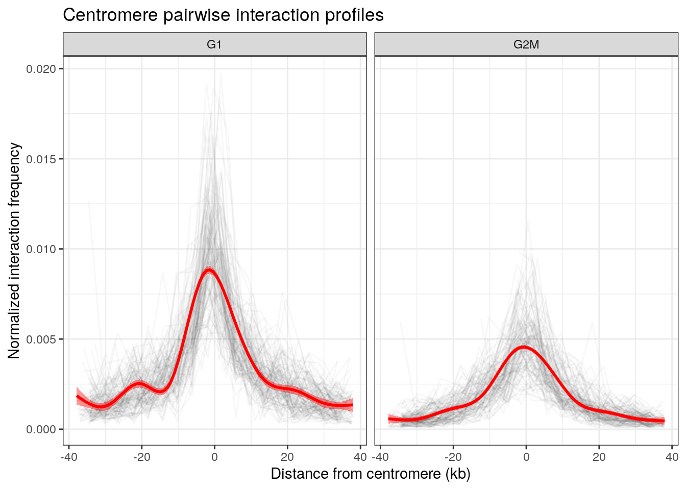
Session info
Click to expand 👇
sessioninfo::session_info(include_base = TRUE)
##  ─ Session info ────────────────────────────────────────────────────────────
##   setting  value
##   version  R Under development (unstable) (2024-01-17 r85813)
##   os       Ubuntu 22.04.3 LTS
##   system   x86_64, linux-gnu
##   ui       X11
##   language (EN)
##   collate  C
##   ctype    en_US.UTF-8
##   tz       Etc/UTC
##   date     2024-01-22
##   pandoc   3.1.1 @ /usr/local/bin/ (via rmarkdown)
##
##  ─ Packages ────────────────────────────────────────────────────────────────
##   package              * version   date (UTC) lib source
##   abind                  1.4-5     2016-07-21 [2] CRAN (R 4.4.0)
##   aggregation            1.0.1     2018-01-25 [2] CRAN (R 4.4.0)
##   AnnotationDbi          1.65.2    2023-11-03 [2] Bioconductor
##   AnnotationHub        * 3.11.1    2023-12-11 [2] Bioconductor 3.19 (R 4.4.0)
##   base                 * 4.4.0     2024-01-18 [3] local
##   beeswarm               0.4.0     2021-06-01 [2] CRAN (R 4.4.0)
##   Biobase              * 2.63.0    2023-10-24 [2] Bioconductor
##   BiocFileCache        * 2.11.1    2023-10-26 [2] Bioconductor
##   BiocGenerics         * 0.49.1    2023-11-01 [2] Bioconductor
##   BiocIO                 1.13.0    2023-10-24 [2] Bioconductor
##   BiocManager            1.30.22   2023-08-08 [2] CRAN (R 4.4.0)
##   BiocParallel           1.37.0    2023-10-24 [2] Bioconductor
##   BiocVersion            3.19.1    2023-10-26 [2] Bioconductor
##   Biostrings             2.71.1    2023-10-25 [2] Bioconductor
##   bit                    4.0.5     2022-11-15 [2] CRAN (R 4.4.0)
##   bit64                  4.0.5     2020-08-30 [2] CRAN (R 4.4.0)
##   bitops                 1.0-7     2021-04-24 [2] CRAN (R 4.4.0)
##   blob                   1.2.4     2023-03-17 [2] CRAN (R 4.4.0)
##   cachem                 1.0.8     2023-05-01 [2] CRAN (R 4.4.0)
##   Cairo                  1.6-2     2023-11-28 [2] CRAN (R 4.4.0)
##   calibrate              1.7.7     2020-06-19 [2] CRAN (R 4.4.0)
##   cli                    3.6.2     2023-12-11 [2] CRAN (R 4.4.0)
##   codetools              0.2-19    2023-02-01 [3] CRAN (R 4.4.0)
##   colorspace             2.1-0     2023-01-23 [2] CRAN (R 4.4.0)
##   compiler               4.4.0     2024-01-18 [3] local
##   cowplot                1.1.2     2023-12-15 [2] CRAN (R 4.4.0)
##   crayon                 1.5.2     2022-09-29 [2] CRAN (R 4.4.0)
##   curl                   5.2.0     2023-12-08 [2] CRAN (R 4.4.0)
##   data.table             1.14.10   2023-12-08 [2] CRAN (R 4.4.0)
##   datasets             * 4.4.0     2024-01-18 [3] local
##   DBI                    1.2.1     2024-01-12 [2] CRAN (R 4.4.0)
##   dbplyr               * 2.4.0     2023-10-26 [2] CRAN (R 4.4.0)
##   DelayedArray           0.29.0    2023-10-24 [2] Bioconductor
##   digest                 0.6.34    2024-01-11 [2] CRAN (R 4.4.0)
##   dplyr                * 1.1.4     2023-11-17 [2] CRAN (R 4.4.0)
##   edgeR                  4.1.11    2024-01-18 [2] Bioconductor 3.19 (R 4.4.0)
##   evaluate               0.23      2023-11-01 [2] CRAN (R 4.4.0)
##   ExperimentHub        * 2.11.1    2023-12-11 [2] Bioconductor 3.19 (R 4.4.0)
##   fansi                  1.0.6     2023-12-08 [2] CRAN (R 4.4.0)
##   farver                 2.1.1     2022-07-06 [2] CRAN (R 4.4.0)
##   fastmap                1.1.1     2023-02-24 [2] CRAN (R 4.4.0)
##   filelock               1.0.3     2023-12-11 [2] CRAN (R 4.4.0)
##   generics               0.1.3     2022-07-05 [2] CRAN (R 4.4.0)
##   GenomeInfoDb         * 1.39.5    2024-01-01 [2] Bioconductor 3.19 (R 4.4.0)
##   GenomeInfoDbData       1.2.11    2024-01-22 [2] Bioconductor
##   GenomicRanges        * 1.55.1    2023-10-29 [2] Bioconductor
##   ggbeeswarm             0.7.2     2023-04-29 [2] CRAN (R 4.4.0)
##   ggplot2              * 3.4.4     2023-10-12 [2] CRAN (R 4.4.0)
##   ggrastr                1.0.2     2023-06-01 [2] CRAN (R 4.4.0)
##   glue                   1.7.0     2024-01-09 [2] CRAN (R 4.4.0)
##   graphics             * 4.4.0     2024-01-18 [3] local
##   grDevices            * 4.4.0     2024-01-18 [3] local
##   grid                   4.4.0     2024-01-18 [3] local
##   gridExtra              2.3       2017-09-09 [2] CRAN (R 4.4.0)
##   gtable                 0.3.4     2023-08-21 [2] CRAN (R 4.4.0)
##   gtools                 3.9.5     2023-11-20 [2] CRAN (R 4.4.0)
##   HiCcompare             1.25.0    2023-10-24 [2] Bioconductor
##   HiCExperiment        * 1.3.0     2023-10-24 [2] Bioconductor
##   HiContacts           * 1.5.0     2023-10-24 [2] Bioconductor
##   HiContactsData       * 1.5.3     2024-01-22 [2] Github (js2264/HiContactsData@d5bebe7)
##   hms                    1.1.3     2023-03-21 [2] CRAN (R 4.4.0)
##   htmltools              0.5.7     2023-11-03 [2] CRAN (R 4.4.0)
##   htmlwidgets            1.6.4     2023-12-06 [2] CRAN (R 4.4.0)
##   httr                   1.4.7     2023-08-15 [2] CRAN (R 4.4.0)
##   InteractionSet       * 1.31.0    2023-10-24 [2] Bioconductor
##   IRanges              * 2.37.1    2024-01-19 [2] Bioconductor 3.19 (R 4.4.0)
##   jsonlite               1.8.8     2023-12-04 [2] CRAN (R 4.4.0)
##   KEGGREST               1.43.0    2023-10-24 [2] Bioconductor
##   KernSmooth             2.23-22   2023-07-10 [3] CRAN (R 4.4.0)
##   knitr                  1.45      2023-10-30 [2] CRAN (R 4.4.0)
##   labeling               0.4.3     2023-08-29 [2] CRAN (R 4.4.0)
##   lattice                0.22-5    2023-10-24 [3] CRAN (R 4.4.0)
##   lifecycle              1.0.4     2023-11-07 [2] CRAN (R 4.4.0)
##   limma                  3.59.1    2023-10-30 [2] Bioconductor
##   locfit                 1.5-9.8   2023-06-11 [2] CRAN (R 4.4.0)
##   magrittr               2.0.3     2022-03-30 [2] CRAN (R 4.4.0)
##   MASS                   7.3-60.2  2024-01-18 [3] local
##   Matrix                 1.6-5     2024-01-11 [3] CRAN (R 4.4.0)
##   MatrixGenerics       * 1.15.0    2023-10-24 [2] Bioconductor
##   matrixStats          * 1.2.0     2023-12-11 [2] CRAN (R 4.4.0)
##   memoise                2.0.1     2021-11-26 [2] CRAN (R 4.4.0)
##   methods              * 4.4.0     2024-01-18 [3] local
##   mgcv                   1.9-1     2023-12-21 [3] CRAN (R 4.4.0)
##   mime                   0.12      2021-09-28 [2] CRAN (R 4.4.0)
##   multiHiCcompare      * 1.21.0    2023-10-24 [2] Bioconductor
##   munsell                0.5.0     2018-06-12 [2] CRAN (R 4.4.0)
##   nlme                   3.1-164   2023-11-27 [3] CRAN (R 4.4.0)
##   parallel               4.4.0     2024-01-18 [3] local
##   pbapply                1.7-2     2023-06-27 [2] CRAN (R 4.4.0)
##   pheatmap               1.0.12    2019-01-04 [2] CRAN (R 4.4.0)
##   pillar                 1.9.0     2023-03-22 [2] CRAN (R 4.4.0)
##   pkgconfig              2.0.3     2019-09-22 [2] CRAN (R 4.4.0)
##   png                    0.1-8     2022-11-29 [2] CRAN (R 4.4.0)
##   purrr                * 1.0.2     2023-08-10 [2] CRAN (R 4.4.0)
##   qqman                  0.1.9     2023-08-23 [2] CRAN (R 4.4.0)
##   R6                     2.5.1     2021-08-19 [2] CRAN (R 4.4.0)
##   rappdirs               0.3.3     2021-01-31 [2] CRAN (R 4.4.0)
##   RColorBrewer           1.1-3     2022-04-03 [2] CRAN (R 4.4.0)
##   Rcpp                   1.0.12    2024-01-09 [2] CRAN (R 4.4.0)
##   RCurl                  1.98-1.14 2024-01-09 [2] CRAN (R 4.4.0)
##   readr                  2.1.5     2024-01-10 [2] CRAN (R 4.4.0)
##   rhdf5                  2.47.2    2024-01-15 [2] Bioconductor 3.19 (R 4.4.0)
##   rhdf5filters           1.15.1    2023-11-06 [2] Bioconductor
##   Rhdf5lib               1.25.1    2023-12-11 [2] Bioconductor 3.19 (R 4.4.0)
##   rlang                  1.1.3     2024-01-10 [2] CRAN (R 4.4.0)
##   rmarkdown              2.25      2023-09-18 [2] CRAN (R 4.4.0)
##   RSpectra               0.16-1    2022-04-24 [2] CRAN (R 4.4.0)
##   RSQLite                2.3.5     2024-01-21 [2] CRAN (R 4.4.0)
##   S4Arrays               1.3.2     2024-01-14 [2] Bioconductor 3.19 (R 4.4.0)
##   S4Vectors            * 0.41.3    2024-01-01 [2] Bioconductor 3.19 (R 4.4.0)
##   scales                 1.3.0     2023-11-28 [2] CRAN (R 4.4.0)
##   sessioninfo            1.2.2     2021-12-06 [2] CRAN (R 4.4.0)
##   SparseArray            1.3.3     2024-01-14 [2] Bioconductor 3.19 (R 4.4.0)
##   splines                4.4.0     2024-01-18 [3] local
##   statmod                1.5.0     2023-01-06 [2] CRAN (R 4.4.0)
##   stats                * 4.4.0     2024-01-18 [3] local
##   stats4               * 4.4.0     2024-01-18 [3] local
##   strawr                 0.0.91    2023-03-29 [2] CRAN (R 4.4.0)
##   stringi                1.8.3     2023-12-11 [2] CRAN (R 4.4.0)
##   stringr                1.5.1     2023-11-14 [2] CRAN (R 4.4.0)
##   SummarizedExperiment * 1.33.2    2024-01-07 [2] Bioconductor 3.19 (R 4.4.0)
##   tibble                 3.2.1     2023-03-20 [2] CRAN (R 4.4.0)
##   tidyr                  1.3.0     2023-01-24 [2] CRAN (R 4.4.0)
##   tidyselect             1.2.0     2022-10-10 [2] CRAN (R 4.4.0)
##   tools                  4.4.0     2024-01-18 [3] local
##   tzdb                   0.4.0     2023-05-12 [2] CRAN (R 4.4.0)
##   utf8                   1.2.4     2023-10-22 [2] CRAN (R 4.4.0)
##   utils                * 4.4.0     2024-01-18 [3] local
##   vctrs                  0.6.5     2023-12-01 [2] CRAN (R 4.4.0)
##   vipor                  0.4.7     2023-12-18 [2] CRAN (R 4.4.0)
##   vroom                  1.6.5     2023-12-05 [2] CRAN (R 4.4.0)
##   withr                  3.0.0     2024-01-16 [2] CRAN (R 4.4.0)
##   xfun                   0.41      2023-11-01 [2] CRAN (R 4.4.0)
##   XVector                0.43.1    2024-01-10 [2] Bioconductor 3.19 (R 4.4.0)
##   yaml                   2.3.8     2023-12-11 [2] CRAN (R 4.4.0)
##   zlibbioc               1.49.0    2023-10-24 [2] Bioconductor
##
##   [1] /tmp/Rtmpq5g2WV/Rinstb37571687
##   [2] /usr/local/lib/R/site-library
##   [3] /usr/local/lib/R/library
##
##  ───────────────────────────────────────────────────────────────────────────