7 Finding topological features in Hi-C

Aims

This chapter focuses on the annotation of topological features from Hi-C contact maps, including:

Chromosome compartments
Topologically associating domains
Stable chromatin loops

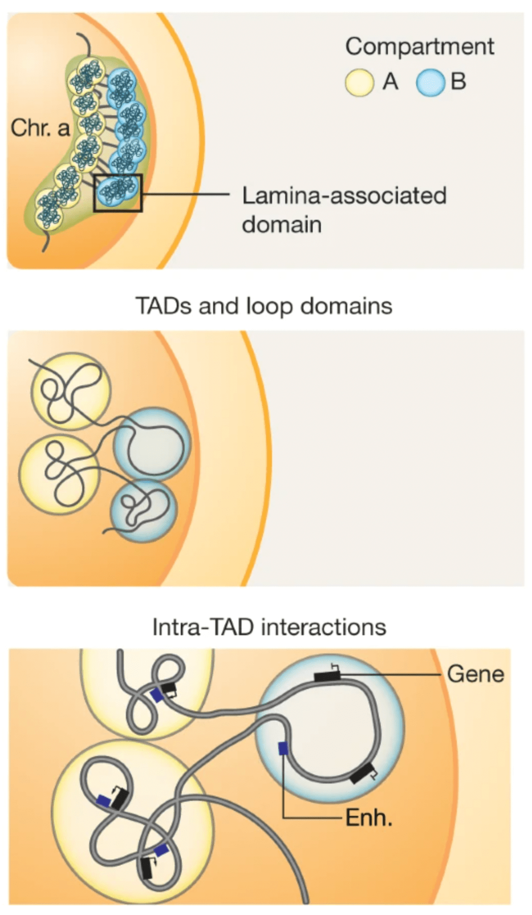
7.1 Chromosome compartments

Chromosome compartments refer to the segregation of the chromatin into active euchromatin (A compartments) and regulated heterochromatin (B compartment).

7.1.1 Importing Hi-C data

To investigate chromosome compartments, we will fetch a contact matrix generated from a micro-C experiment (from Krietenstein et al. (2020)). A subset of the genome-wide dataset is provided in the HiContactsData package. It contains intra-chromosomal interactions within chr17, binned at 5000, 100000 and 250000 bp.

library(HiCExperiment)
library(HiContactsData)
cf <- CoolFile(HiContactsData('microC', 'mcool'))
##  see ?HiContactsData and browseVignettes('HiContactsData') for documentation
##  downloading 1 resources
##  retrieving 1 resource
##  loading from cache
microC <- import(cf, resolution = 250000)
microC
##  `HiCExperiment` object with 10,086,710 contacts over 334 regions 
##  -------
##  fileName: "/root/.cache/R/ExperimentHub/145c1451bdc6_8601" 
##  focus: "whole genome" 
##  resolutions(3): 5000 100000 250000
##  active resolution: 250000 
##  interactions: 52755 
##  scores(2): count balanced 
##  topologicalFeatures: compartments(0) borders(0) loops(0) viewpoints(0) 
##  pairsFile: N/A 
##  metadata(0):

seqinfo(microC)
##  Seqinfo object with 1 sequence from an unspecified genome:
##    seqnames seqlengths isCircular genome
##    chr17      83257441         NA   <NA>

7.1.2 Annotating A/B compartments

The consensus approach to annotate A/B compartments is to compute the eigenvectors of a Hi-C contact matrix and identify the eigenvector representing the chromosome-wide bi-partite segmentation of the genome.

The getCompartments() function performs several internal operations to achieve this:

Obtains cis interactions per chromosome
Computes O/E contact matrix scores
Computes 3 first eigenvectors of this Hi-C contact matrix
Normalizes eigenvectors
Picks the eigenvector that has the greatest absolute correlation with a phasing track (e.g. a GC% track automatically computed from a genome reference sequence, or a gene density track)
Signs this eigenvector so that positive values represent the A compartment

phasing_track <- BSgenome.Hsapiens.UCSC.hg38::BSgenome.Hsapiens.UCSC.hg38
microC_compts <- getCompartments(microC, genome = phasing_track)
##  Going through preflight checklist...
##  Parsing intra-chromosomal contacts for each chromosome...
##  Computing eigenvectors for each chromosome...

microC_compts
##  `HiCExperiment` object with 10,086,710 contacts over 334 regions 
##  -------
##  fileName: "/root/.cache/R/ExperimentHub/145c1451bdc6_8601" 
##  focus: "whole genome" 
##  resolutions(3): 5000 100000 250000
##  active resolution: 250000 
##  interactions: 52755 
##  scores(2): count balanced 
##  topologicalFeatures: compartments(41) borders(0) loops(0) viewpoints(0) 
##  pairsFile: N/A 
##  metadata(1): eigens

getCompartments() is an endomorphism: it returns the original object, enriched with two new pieces of information:

A compartments topologicalFeatures:

topologicalFeatures(microC_compts, "compartments")
##  GRanges object with 41 ranges and 1 metadata column:
##         seqnames            ranges strand | compartment
##            <Rle>         <IRanges>  <Rle> | <character>
##     [1]    chr17    250001-3000000      * |           A
##     [2]    chr17   3000001-3500000      * |           B
##     [3]    chr17   3500001-5500000      * |           A
##     [4]    chr17   5500001-6500000      * |           B
##     [5]    chr17   6500001-8500000      * |           A
##     ...      ...               ...    ... .         ...
##    [37]    chr17 72750001-73250000      * |           A
##    [38]    chr17 73250001-74750000      * |           B
##    [39]    chr17 74750001-79250000      * |           A
##    [40]    chr17 79250001-79750000      * |           B
##    [41]    chr17 79750001-83250000      * |           A
##    -------
##    seqinfo: 1 sequence from an unspecified genome

The calculated eigenvectors stored in metadata:

metadata(microC_compts)$eigens
##  GRanges object with 334 ranges and 9 metadata columns:
##                                  seqnames            ranges strand |
##                                     <Rle>         <IRanges>  <Rle> |
##             chr17.chr17_1_250000    chr17          1-250000      * |
##        chr17.chr17_250001_500000    chr17     250001-500000      * |
##        chr17.chr17_500001_750000    chr17     500001-750000      * |
##       chr17.chr17_750001_1000000    chr17    750001-1000000      * |
##      chr17.chr17_1000001_1250000    chr17   1000001-1250000      * |
##                              ...      ...               ...    ... .
##    chr17.chr17_82250001_82500000    chr17 82250001-82500000      * |
##    chr17.chr17_82500001_82750000    chr17 82500001-82750000      * |
##    chr17.chr17_82750001_83000000    chr17 82750001-83000000      * |
##    chr17.chr17_83000001_83250000    chr17 83000001-83250000      * |
##    chr17.chr17_83250001_83257441    chr17 83250001-83257441      * |
##                                     bin_id     weight   chr    center
##                                  <numeric>  <numeric> <Rle> <integer>
##             chr17.chr17_1_250000         0        NaN chr17    125000
##        chr17.chr17_250001_500000         1 0.00626903 chr17    375000
##        chr17.chr17_500001_750000         2 0.00567190 chr17    625000
##       chr17.chr17_750001_1000000         3 0.00528588 chr17    875000
##      chr17.chr17_1000001_1250000         4 0.00464628 chr17   1125000
##                              ...       ...        ...   ...       ...
##    chr17.chr17_82250001_82500000       329 0.00463044 chr17  82375000
##    chr17.chr17_82500001_82750000       330 0.00486910 chr17  82625000
##    chr17.chr17_82750001_83000000       331 0.00561269 chr17  82875000
##    chr17.chr17_83000001_83250000       332 0.00546433 chr17  83125000
##    chr17.chr17_83250001_83257441       333        NaN chr17  83253721
##                                         E1        E2        E3   phasing
##                                  <numeric> <numeric> <numeric> <numeric>
##             chr17.chr17_1_250000  0.000000  0.000000  0.000000  0.383084
##        chr17.chr17_250001_500000  0.450991  0.653287  0.615300  0.433972
##        chr17.chr17_500001_750000  0.716784  0.707461  0.845033  0.465556
##       chr17.chr17_750001_1000000  0.904423  0.414952  0.864288  0.503592
##      chr17.chr17_1000001_1250000  0.913023  0.266287  0.759016  0.547712
##                              ...       ...       ...       ...       ...
##    chr17.chr17_82250001_82500000  1.147060  0.239112  1.133498  0.550872
##    chr17.chr17_82500001_82750000  1.106937  0.419647  1.169464  0.513212
##    chr17.chr17_82750001_83000000  0.818990  0.591955  0.850340  0.522432
##    chr17.chr17_83000001_83250000  0.874038  0.503175  0.847926  0.528448
##    chr17.chr17_83250001_83257441  0.000000  0.000000  0.000000  0.000000
##                                      eigen
##                                  <numeric>
##             chr17.chr17_1_250000  0.000000
##        chr17.chr17_250001_500000  0.450991
##        chr17.chr17_500001_750000  0.716784
##       chr17.chr17_750001_1000000  0.904423
##      chr17.chr17_1000001_1250000  0.913023
##                              ...       ...
##    chr17.chr17_82250001_82500000  1.147060
##    chr17.chr17_82500001_82750000  1.106937
##    chr17.chr17_82750001_83000000  0.818990
##    chr17.chr17_83000001_83250000  0.874038
##    chr17.chr17_83250001_83257441  0.000000
##    -------
##    seqinfo: 1 sequence from an unspecified genome

7.1.3 Exporting compartment tracks

To save the eigenvector (as a bigwig file) and the compartments(as a gff file), the export function can be used:

library(GenomicRanges)
library(rtracklayer)
coverage(metadata(microC_compts)$eigens, weight = 'eigen') |> export('microC_eigen.bw')
topologicalFeatures(microC_compts, "compartments") |> export('microC_compartments.gff3')

7.1.4 Visualizing compartment tracks

Compartment tracks should be visualized in a dedicated genome browser, with the phasing track loaded as well, to ensure they are phased accordingly.
That being said, it is possible to visualize a genome track in R besides the matching Hi-C contact matrix.

library(ggplot2)
library(patchwork)
microC <- autocorrelate(microC)
##  
p1 <- plotMatrix(microC, use.scores = 'autocorrelated', scale = 'linear', limits = c(-1, 1), caption = FALSE)
eigen <- coverage(metadata(microC_compts)$eigens, weight = 'eigen')[[1]]
eigen_df <- tibble(pos = cumsum(runLength(eigen)), eigen = runValue(eigen))
p2 <- ggplot(eigen_df, aes(x = pos, y = eigen)) + 
    geom_area() + 
    theme_void() + 
    coord_cartesian(expand = FALSE) + 
    labs(x = "Genomic position", y = "Eigenvector value")
wrap_plots(p1, p2, ncol = 1, heights = c(10, 1))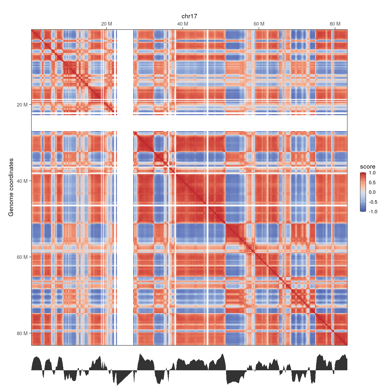

Here, we clearly note the concordance between the Hi-C correlation matrix, highlighting correlated interactions between pairs of genomic segments, and the eigenvector representing chromosome segmentation into 2 compartments: A (for positive values) and B (for negative values).

7.1.5 Saddle plots

Saddle plots are typically used to measure the observed vs. expected interaction scores within or between genomic loci belonging to A and B compartments.

Non-overlapping genomic windows are grouped in nbins quantiles (typically between 10 and 50 quantiles) according to their A/B compartment eigenvector value, from lowest eigenvector values (i.e. strongest B compartments) to highest eigenvector values (i.e. strongest A compartments). The average observed vs. expected interaction scores are then computed for pairwise eigenvector quantiles and plotted in a 2D heatmap.

library(BiocParallel)
plotSaddle(microC_compts, nbins = 25, BPPARAM = SerialParam(progressbar = FALSE))

Here, the top-left small corner represents average O/E scores between strong B compartments and the bottom-right larger corner represents average O/E scores between strong A compartments. Note that only chr17 interactions are contained in this dataset, explaining the grainy aspect of the saddle plot.

7.2 Topological domains

Topological domains (a.k.a. Topologically Associating Domains, TADs, isolated neighborhoods, contact domains, …) refer to local chromosomal segments (e.b. roughly ≤ 1Mb in mammal genomes) which preferentially self-interact, in a constrained manner. They are demarcated by domain boundaries.

They are generally conserved across cell types and species (Schmitt et al. (2016)), typically correlate with units of DNA replication (Pope et al. (2014)), and could play a role during development (Stadhouders et al. (2019)).

7.2.1 Computing diamond insulation score

Several approaches exist to annotate topological domains (Sefer (2022)). Several packages in R implement some of these functionalities, e.g. spectralTAD or TADcompare.

HiContacts offers a simple getDiamondInsulation function which computes the diamond insulation score (Crane et al. (2015)). This score quantifies average interaction frequency in an insulation window (of a certain window_size) sliding along contact matrices at a chosen resolution.

# - Compute insulation score
bpparam <- SerialParam(progressbar = FALSE)
hic <- zoom(microC, 5000) |> 
    refocus('chr17:60000001-83257441') |>
    getDiamondInsulation(window_size = 100000, BPPARAM = bpparam) |> 
    getBorders()
##  Going through preflight checklist...
##  Scan each window and compute diamond insulation score...
##  Annotating diamond score prominence for each window...

hic
##  `HiCExperiment` object with 2,156,222 contacts over 4,652 regions 
##  -------
##  fileName: "/root/.cache/R/ExperimentHub/145c1451bdc6_8601" 
##  focus: "chr17:60,000,001-83,257,441" 
##  resolutions(3): 5000 100000 250000
##  active resolution: 5000 
##  interactions: 2156044 
##  scores(2): count balanced 
##  topologicalFeatures: compartments(0) borders(21) loops(0) viewpoints(0) 
##  pairsFile: N/A 
##  metadata(1): insulation

getDiamondInsulation() is an endomorphism: it returns the original object, enriched with two new pieces of information:

A borders topologicalFeatures:

topologicalFeatures(hic, "borders")
##  GRanges object with 21 ranges and 1 metadata column:
##           seqnames            ranges strand |     score
##              <Rle>         <IRanges>  <Rle> | <numeric>
##    strong    chr17 60105001-60110000      * |  0.574760
##      weak    chr17 60210001-60215000      * |  0.414425
##      weak    chr17 61415001-61420000      * |  0.346668
##    strong    chr17 61500001-61505000      * |  0.544336
##      weak    chr17 62930001-62935000      * |  0.399794
##       ...      ...               ...    ... .       ...
##      weak    chr17 78395001-78400000      * |  0.235613
##      weak    chr17 79065001-79070000      * |  0.236535
##      weak    chr17 80155001-80160000      * |  0.284855
##      weak    chr17 81735001-81740000      * |  0.497478
##    strong    chr17 81840001-81845000      * |  1.395949
##    -------
##    seqinfo: 1 sequence from an unspecified genome

The calculated insulation scores stored in metadata:

metadata(hic)$insulation
##  GRanges object with 4611 ranges and 8 metadata columns:
##                            seqnames            ranges strand |    bin_id
##                               <Rle>         <IRanges>  <Rle> | <numeric>
##    chr17_60100001_60105000    chr17 60100001-60105000      * |     12020
##    chr17_60105001_60110000    chr17 60105001-60110000      * |     12021
##    chr17_60110001_60115000    chr17 60110001-60115000      * |     12022
##    chr17_60115001_60120000    chr17 60115001-60120000      * |     12023
##    chr17_60120001_60125000    chr17 60120001-60125000      * |     12024
##                        ...      ...               ...    ... .       ...
##    chr17_83130001_83135000    chr17 83130001-83135000      * |     16626
##    chr17_83135001_83140000    chr17 83135001-83140000      * |     16627
##    chr17_83140001_83145000    chr17 83140001-83145000      * |     16628
##    chr17_83145001_83150000    chr17 83145001-83150000      * |     16629
##    chr17_83150001_83155000    chr17 83150001-83155000      * |     16630
##                               weight   chr    center     score insulation
##                            <numeric> <Rle> <integer> <numeric>  <numeric>
##    chr17_60100001_60105000 0.0406489 chr17  60102500  0.188061  -0.750142
##    chr17_60105001_60110000 0.0255539 chr17  60107500  0.180860  -0.806466
##    chr17_60110001_60115000       NaN chr17  60112500  0.196579  -0.686232
##    chr17_60115001_60120000       NaN chr17  60117500  0.216039  -0.550046
##    chr17_60120001_60125000       NaN chr17  60122500  0.230035  -0.459489
##                        ...       ...   ...       ...       ...        ...
##    chr17_83130001_83135000 0.0314684 chr17  83132500  0.262191  -0.270723
##    chr17_83135001_83140000 0.0307197 chr17  83137500  0.240779  -0.393632
##    chr17_83140001_83145000 0.0322810 chr17  83142500  0.219113  -0.529664
##    chr17_83145001_83150000 0.0280840 chr17  83147500  0.199645  -0.663900
##    chr17_83150001_83155000 0.0272775 chr17  83152500  0.180434  -0.809873
##                                  min prominence
##                            <logical>  <numeric>
##    chr17_60100001_60105000     FALSE         NA
##    chr17_60105001_60110000      TRUE    0.57476
##    chr17_60110001_60115000     FALSE         NA
##    chr17_60115001_60120000     FALSE         NA
##    chr17_60120001_60125000     FALSE         NA
##                        ...       ...        ...
##    chr17_83130001_83135000     FALSE         NA
##    chr17_83135001_83140000     FALSE         NA
##    chr17_83140001_83145000     FALSE         NA
##    chr17_83145001_83150000     FALSE         NA
##    chr17_83150001_83155000     FALSE         NA
##    -------
##    seqinfo: 1 sequence from an unspecified genome

Note

The getDiamondInsulation function can be parallelized over multiple threads by specifying the Bioconductor generic BPPARAM argument.

7.2.2 Exporting insulation scores tracks

To save the diamond insulation scores (as a bigwig file) and the borders (as a bed file), the export function can be used:

coverage(metadata(hic)$insulation, weight = 'insulation') |> export('microC_insulation.bw')
topologicalFeatures(hic, "borders") |> export('microC_borders.bed')

7.2.3 Visualizing chromatin domains

Insulation tracks should be visualized in a dedicated genome browser.
That being said, it is possible to visualize a genome track in R besides the matching Hi-C contact matrix.

hic <- zoom(hic, 100000)
p1 <- plotMatrix(
    hic, 
    use.scores = 'balanced', 
    limits = c(-3.5, -1),
    borders = topologicalFeatures(hic, "borders"),
    caption = FALSE
)
insulation <- coverage(metadata(hic)$insulation, weight = 'insulation')[[1]]
insulation_df <- tibble(pos = cumsum(runLength(insulation)), insulation = runValue(insulation))
p2 <- ggplot(insulation_df, aes(x = pos, y = insulation)) + 
    geom_area() + 
    theme_void() + 
    coord_cartesian(expand = FALSE) + 
    labs(x = "Genomic position", y = "Diamond insulation score")
wrap_plots(p1, p2, ncol = 1, heights = c(10, 1))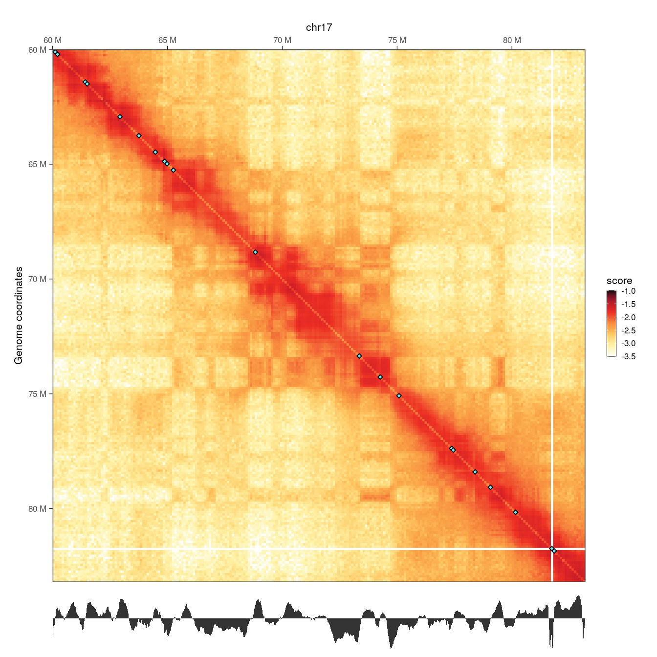

Local minima in the diamond insulation score displayed below the Hi-C contact matrix are identified using the getBorders() function, which automatically estimates a minimum threshold. These local minima correspond to borders and are visually depicted on the Hi-C map by blue diamonds.

7.3 Chromatin loops

7.3.1 `chromosight`

Chromatin loops, dots, or contacts, refer to a strong increase of interaction frequency between a pair of two genomic loci. They correspond to focal “dots” on a Hi-C map. Relying on computer vision algorithms, chromosight uses this property to annotate chromatin loops in a Hi-C map (Matthey-Doret et al. (2020)). chromosight is a standalone python package and is made available in R through the HiCool-managed conda environment with the getLoops() function.

7.3.1.1 Identifying loops

hic <- HiCool::getLoops(microC, resolution = 5000)

hic
## `HiCExperiment` object with 917,156 contacts over 100 regions
## -------
## fileName: "/home/rsg/.cache/R/fourDNData/4d434d8538a0_4DNFI9FVHJZQ.mcool"
## focus: "chr17:63,000,001-63,500,000"
## resolutions(13): 1000 2000 ... 5000000 10000000
## active resolution: 5000
## interactions: 5047
## scores(2): count balanced
## topologicalFeatures: compartments(0) borders(0) loops(66411) viewpoints(0)
## pairsFile: N/A
## metadata(1): chromosight_args

getLoops() is an endomorphism: it returns the original object, enriched with two new pieces of information:

A loops topologicalFeatures:

topologicalFeatures(hic, "loops")
## GInteractions object with 66411 interactions and 5 metadata columns:
##           seqnames1           ranges1     seqnames2           ranges2 |   bin_id1   bin_id2     score      ## pvalue    qvalue
##               <Rle>         <IRanges>         <Rle>         <IRanges> | <numeric> <numeric> <numeric>   ## <numeric> <numeric>
##       [1]      chr1     775001-780000 ---      chr1     850001-855000 |       155       170  0.334586 2.## 15995e-05 2.162e-05
##       [2]      chr1     775001-780000 ---      chr1     865001-870000 |       155       173  0.403336 1.## 62900e-07 1.669e-07
##       [3]      chr1     865001-870000 ---      chr1     890001-895000 |       173       178  0.337344 1.## 91400e-07 1.957e-07
##       [4]      chr1     910001-915000 ---      chr1     955001-960000 |       182       191  0.639725 0.## 00000e+00 0.000e+00
##       [5]      chr1     910001-915000 ---      chr1   1055001-1060000 |       182       211  0.521699 0.## 00000e+00 0.000e+00
##       ...       ...               ... ...       ...               ... .       ...       ...       ...       ##   ...       ...
##   [66407]      chrY 19570001-19575000 ---      chrY 19720001-19725000 |    610133    610163  0.315529    3.## 30e-08  3.55e-08
##   [66408]      chrY 19705001-19710000 ---      chrY 19730001-19735000 |    610160    610165  0.708753    0.## 00e+00  0.00e+00
##   [66409]      chrY 19765001-19770000 ---      chrY 19800001-19805000 |    610172    610179  0.373635    1.## 10e-09  1.40e-09
##   [66410]      chrY 20555001-20560000 ---      chrY 20645001-20650000 |    610330    610348  0.603308    0.## 00e+00  0.00e+00
##   [66411]      chrY 21015001-21020000 ---      chrY 21055001-21060000 |    610422    610430  0.394614    9.## 12e-08  9.45e-08
##   -------
##   regions: 84171 ranges and 0 metadata columns
##   seqinfo: 24 sequences from an unspecified genome; no seqlengths

The arguments used by chromosight, stored in metadata:

metadata(hic)$chromosight_args
## $`--pattern`
## [1] "loops"
## 
## $`--dump`
## [1] "/data/.cache/R//RtmpSaRwiZ"
## 
## $`--inter`
## [1] FALSE
## 
## $`--iterations`
## [1] "auto"
## 
## $`--kernel-config`
## NULL
## 
## $`--perc-zero`
## [1] "auto"
## 
## $`--perc-undetected`
## [1] "auto"
## 
## $`--tsvd`
## [1] FALSE
## 
## $`--win-fmt`
## [1] "json"
## 
## $`--win-size`
## [1] "auto"
## 
## $`--no-plotting`
## [1] TRUE
## 
## $`--smooth-trend`
## [1] FALSE
## 
## $`--norm`
## [1] "auto"
## 
## $`<contact_map>`
## [1] "/home/rsg/.cache/R/fourDNData/4d434d8538a0_4DNFI9FVHJZQ.mcool::/resolutions/5000"
## 
## $`--max-dist`
## [1] "auto"
## 
## $`--min-dist`
## [1] "auto"
## 
## $`--min-separation`
## [1] "auto"
## 
## $`--n-mads`
## [1] 5
## 
## $`<prefix>`
## [1] "chromosight/chromo"
## 
## $`--pearson`
## [1] "auto"
## 
## $`--subsample`
## [1] "no"
## 
## $`--threads`
## [1] 1

7.3.1.2 Importing loops from files

If you are using chromosight directly from the terminal (i.e. outside R), you can import the annotated loops in R as follows:

df <- readr::read_tsv("...") ## Here put your loops file
loops <- InteractionSet::GInteractions(
    anchor1 = GenomicRanges::GRanges(
        df$chrom1, IRanges::IRanges(df$start1+1, df$end1)
    ),
    anchor2 = GenomicRanges::GRanges(
        df$chrom2, IRanges::IRanges(df$start2+1, df$end2)
    ),
    bin_id1 = df$bin1, 
    bin_id2 = df$bin2, 
    score = df$score, 
    pvalue = df$pvalue, 
    qvalue = df$qvalue
)

7.3.1.3 Exporting chromatin loops

loops <- topologicalFeatures(hic, "loops")
loops <- loops[loops$score >= 0.4 & loops$qvalue <= 1e-6]
GenomicInteractions::export.bedpe(loops, 'loops.bedpe')

7.3.1.4 Visualizing chromatin loops

plotMatrix(
    refocus(hic, 'chr17:62500001-63500000') |> zoom(5000), 
    loops = loops,
    limits = c(-4, -1.2),
    caption = FALSE
)

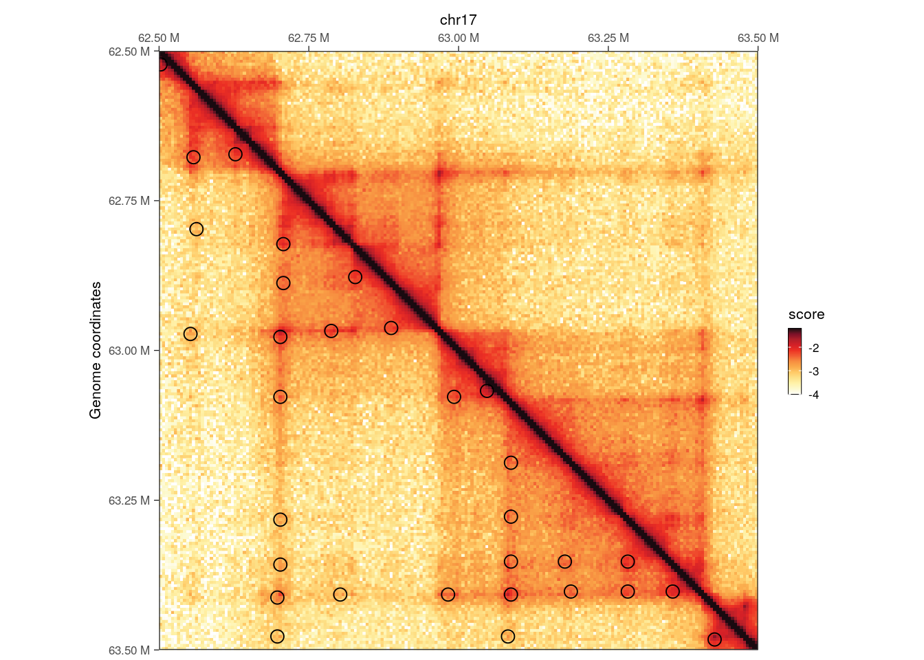
7.3.2 Other R packages

A number of other R packages have been developed to identify focal chromatin loops, notably fitHiC (Ay et al. (2014)), GOTHiC (Mifsud et al. (2017)) or idr2d (Krismer et al. (2020)). Each fits a slightly different purpose, and we encourage the end user to read companion publications.

References

Ay, F., Bailey, T. L., & Noble, W. S. (2014). Statistical confidence estimation for hi-c data reveals regulatory chromatin contacts. Genome Research, 24(6), 999–1011. https://doi.org/10.1101/gr.160374.113

Crane, E., Bian, Q., McCord, R. P., Lajoie, B. R., Wheeler, B. S., Ralston, E. J., Uzawa, S., Dekker, J., & Meyer, B. J. (2015). Condensin-driven remodelling of x chromosome topology during dosage compensation. Nature, 523(7559), 240–244. https://doi.org/10.1038/nature14450

Krietenstein, N., Abraham, S., Venev, S. V., Abdennur, N., Gibcus, J., Hsieh, T.-H. S., Parsi, K. M., Yang, L., Maehr, R., Mirny, L. A., Dekker, J., & Rando, O. J. (2020). Ultrastructural details of mammalian chromosome architecture. Molecular Cell, 78(3), 554–565.e7. https://doi.org/10.1016/j.molcel.2020.03.003

Krismer, K., Guo, Y., & Gifford, D. K. (2020). IDR2D identifies reproducible genomic interactions. Nucleic Acids Research, 48(6), e31–e31. https://doi.org/10.1093/nar/gkaa030

Matthey-Doret, C., Baudry, L., Breuer, A., Montagne, R., Guiglielmoni, N., Scolari, V., Jean, E., Campeas, A., Chanut, P. H., Oriol, E., Méot, A., Politis, L., Vigouroux, A., Moreau, P., Koszul, R., & Cournac, A. (2020). Computer vision for pattern detection in chromosome contact maps. Nature Communications, 11(1). https://doi.org/10.1038/s41467-020-19562-7

Mifsud, B., Martincorena, I., Darbo, E., Sugar, R., Schoenfelder, S., Fraser, P., & Luscombe, N. M. (2017). GOTHiC, a probabilistic model to resolve complex biases and to identify real interactions in hi-c data. PLOS ONE, 12(4), e0174744. https://doi.org/10.1371/journal.pone.0174744

Pope, B. D., Ryba, T., Dileep, V., Yue, F., Wu, W., Denas, O., Vera, D. L., Wang, Y., Hansen, R. S., Canfield, T. K., Thurman, R. E., Cheng, Y., Gülsoy, G., Dennis, J. H., Snyder, M. P., Stamatoyannopoulos, J. A., Taylor, J., Hardison, R. C., Kahveci, T., … Gilbert, D. M. (2014). Topologically associating domains are stable units of replication-timing regulation. Nature, 515(7527), 402–405. https://doi.org/10.1038/nature13986

Schmitt, A. D., Hu, M., Jung, I., Xu, Z., Qiu, Y., Tan, C. L., Li, Y., Lin, S., Lin, Y., Barr, C. L., & Ren, B. (2016). A compendium of chromatin contact maps reveals spatially active regions in the human genome. Cell Reports, 17(8), 2042–2059. https://doi.org/10.1016/j.celrep.2016.10.061

Sefer, E. (2022). A comparison of topologically associating domain callers over mammals at high resolution. BMC Bioinformatics, 23(1). https://doi.org/10.1186/s12859-022-04674-2

Stadhouders, R., Filion, G. J., & Graf, T. (2019). Transcription factors and 3D genome conformation in cell-fate decisions. Nature, 569(7756), 345–354. https://doi.org/10.1038/s41586-019-1182-7

7.1 Chromosome compartments

7.1.1 Importing Hi-C data

7.1.2 Annotating A/B compartments

7.1.3 Exporting compartment tracks

7.1.4 Visualizing compartment tracks

7.1.5 Saddle plots

7.2 Topological domains

7.2.1 Computing diamond insulation score

7.2.2 Exporting insulation scores tracks

7.2.3 Visualizing chromatin domains

7.3 Chromatin loops

7.3.1 chromosight

7.3.1.1 Identifying loops

7.3.1.2 Importing loops from files

7.3.1.3 Exporting chromatin loops

7.3.1.4 Visualizing chromatin loops

7.3.2 Other R packages

References

7.3.1 `chromosight`