Applying tidy principles to investigating chromatin composition and architecture

Manipulating genomic ranges data

Importing `GRanges` from files

Recommended time: 10 min

The BiocIO::import() generic function lets one import bed files (or alike) into GRanges object in R.

library(GenomicRanges)
#> Loading required package: stats4
#> Loading required package: BiocGenerics
#> 
#> Attaching package: 'BiocGenerics'
#> The following objects are masked from 'package:stats':
#> 
#>     IQR, mad, sd, var, xtabs
#> The following objects are masked from 'package:base':
#> 
#>     anyDuplicated, aperm, append, as.data.frame, basename, cbind,
#>     colnames, dirname, do.call, duplicated, eval, evalq, Filter, Find,
#>     get, grep, grepl, intersect, is.unsorted, lapply, Map, mapply,
#>     match, mget, order, paste, pmax, pmax.int, pmin, pmin.int,
#>     Position, rank, rbind, Reduce, rownames, sapply, setdiff, table,
#>     tapply, union, unique, unsplit, which.max, which.min
#> Loading required package: S4Vectors
#> 
#> Attaching package: 'S4Vectors'
#> The following object is masked from 'package:utils':
#> 
#>     findMatches
#> The following objects are masked from 'package:base':
#> 
#>     expand.grid, I, unname
#> Loading required package: IRanges
#> Loading required package: GenomeInfoDb

library(rtracklayer)

bedf <- system.file('extdata', 'S288C-borders.bed', package = 'Bioc2024tidyWorkshop', mustWork = TRUE)

import(bedf)
#> GRanges object with 814 ranges and 0 metadata columns:
#>         seqnames        ranges strand
#>            <Rle>     <IRanges>  <Rle>
#>     [1]        I   73001-74000      *
#>     [2]        I 108001-109000      *
#>     [3]        I 181001-182000      *
#>     [4]       II   90001-91000      *
#>     [5]       II 119001-120000      *
#>     ...      ...           ...    ...
#>   [810]      XVI 777001-778000      *
#>   [811]      XVI 796001-797000      *
#>   [812]      XVI 811001-812000      *
#>   [813]      XVI 890001-891000      *
#>   [814]      XVI 933001-934000      *
#>   -------
#>   seqinfo: 16 sequences from an unspecified genome; no seqlengths

The tidy way of importing genomic ranges in R, however, is to read files as a data.frame (or tibble) and coerce it as a GRanges once it’s imported in memory.

library(tidyverse)
#> ── Attaching core tidyverse packages ──────────────────────── tidyverse 2.0.0 ──
#> ✔ dplyr     1.1.4     ✔ readr     2.1.5
#> ✔ forcats   1.0.0     ✔ stringr   1.5.1
#> ✔ ggplot2   3.5.1     ✔ tibble    3.2.1
#> ✔ lubridate 1.9.3     ✔ tidyr     1.3.1
#> ✔ purrr     1.0.2     
#> ── Conflicts ────────────────────────────────────────── tidyverse_conflicts() ──
#> ✖ lubridate::%within%() masks IRanges::%within%()
#> ✖ dplyr::collapse()     masks IRanges::collapse()
#> ✖ dplyr::combine()      masks BiocGenerics::combine()
#> ✖ dplyr::desc()         masks IRanges::desc()
#> ✖ tidyr::expand()       masks S4Vectors::expand()
#> ✖ dplyr::filter()       masks stats::filter()
#> ✖ dplyr::first()        masks S4Vectors::first()
#> ✖ dplyr::lag()          masks stats::lag()
#> ✖ ggplot2::Position()   masks BiocGenerics::Position(), base::Position()
#> ✖ purrr::reduce()       masks GenomicRanges::reduce(), IRanges::reduce()
#> ✖ dplyr::rename()       masks S4Vectors::rename()
#> ✖ lubridate::second()   masks S4Vectors::second()
#> ✖ lubridate::second<-() masks S4Vectors::second<-()
#> ✖ dplyr::slice()        masks IRanges::slice()
#> ℹ Use the conflicted package (<http://conflicted.r-lib.org/>) to force all conflicts to become errors

tib <- read_tsv(bedf, col_names = FALSE)
#> Rows: 814 Columns: 3
#> ── Column specification ────────────────────────────────────────────────────────
#> Delimiter: "\t"
#> chr (1): X1
#> dbl (2): X2, X3
#> 
#> ℹ Use `spec()` to retrieve the full column specification for this data.
#> ℹ Specify the column types or set `show_col_types = FALSE` to quiet this message.

tib 
#> # A tibble: 814 × 3
#>    X1        X2     X3
#>    <chr>  <dbl>  <dbl>
#>  1 I      73000  74000
#>  2 I     108000 109000
#>  3 I     181000 182000
#>  4 II     90000  91000
#>  5 II    119000 120000
#>  6 II    136000 137000
#>  7 II    141000 142000
#>  8 II    146000 147000
#>  9 II    159000 160000
#> 10 II    198000 199000
#> # ℹ 804 more rows

library(plyranges)
#> 
#> Attaching package: 'plyranges'
#> 
#> The following objects are masked from 'package:dplyr':
#> 
#>     between, n, n_distinct
#> 
#> The following object is masked from 'package:IRanges':
#> 
#>     slice
#> 
#> The following object is masked from 'package:stats':
#> 
#>     filter

gr <- as_granges(tib, seqnames = X1, start = X2, end = X3)

gr
#> GRanges object with 814 ranges and 0 metadata columns:
#>         seqnames        ranges strand
#>            <Rle>     <IRanges>  <Rle>
#>     [1]        I   73000-74000      *
#>     [2]        I 108000-109000      *
#>     [3]        I 181000-182000      *
#>     [4]       II   90000-91000      *
#>     [5]       II 119000-120000      *
#>     ...      ...           ...    ...
#>   [810]      XVI 777000-778000      *
#>   [811]      XVI 796000-797000      *
#>   [812]      XVI 811000-812000      *
#>   [813]      XVI 890000-891000      *
#>   [814]      XVI 933000-934000      *
#>   -------
#>   seqinfo: 16 sequences from an unspecified genome; no seqlengths

Note how refering to column names is done using tidy evaluation.

Manipulating `GRanges` with tidy verbs

Recommended time: 10 min

With plyranges, a number of tidy operations are readily available, e.g.:

Just like with tidyverse functions, these operations work well with the native |> pipe in R.

gr |> 
    mutate(score = runif(n())) |> 
    filter(score > 0.2) |> 
    mutate(round_score = round(score, digits = 1)) |> 
    group_by(round_score) |> 
    summarize(mean = mean(score))
#> DataFrame with 9 rows and 2 columns
#>   round_score      mean
#>     <numeric> <numeric>
#> 1         0.2  0.223774
#> 2         0.3  0.295649
#> 3         0.4  0.395325
#> 4         0.5  0.503838
#> 5         0.6  0.605391
#> 6         0.7  0.696852
#> 7         0.8  0.798926
#> 8         0.9  0.897357
#> 9         1.0  0.976044

But really, what plyranges excels at is providing direct access to “protected” variables, i.e. seqnames, start, end, width, strand, …

gr |> 
    mutate(
        seqnames = factor('XVI', levels(seqnames)), 
        width = 1, 
        strand = rep(c('-', '+'), n()/2)
    )
#> GRanges object with 814 ranges and 0 metadata columns:
#>         seqnames    ranges strand
#>            <Rle> <IRanges>  <Rle>
#>     [1]      XVI     73000      -
#>     [2]      XVI    108000      +
#>     [3]      XVI    181000      -
#>     [4]      XVI     90000      +
#>     [5]      XVI    119000      -
#>     ...      ...       ...    ...
#>   [810]      XVI    777000      +
#>   [811]      XVI    796000      -
#>   [812]      XVI    811000      +
#>   [813]      XVI    890000      -
#>   [814]      XVI    933000      +
#>   -------
#>   seqinfo: 16 sequences from an unspecified genome; no seqlengths

Finally, a number of operations for genomic arithmetics are provided by plyranges:

gr |> 
    anchor_center() |> 
    stretch(extend = -1000) |> 
    shift_upstream(250) |> 
    flank_upstream(100)
#> GRanges object with 814 ranges and 0 metadata columns:
#>         seqnames        ranges strand
#>            <Rle>     <IRanges>  <Rle>
#>     [1]        I   73150-73249      *
#>     [2]        I 108150-108249      *
#>     [3]        I 181150-181249      *
#>     [4]       II   90150-90249      *
#>     [5]       II 119150-119249      *
#>     ...      ...           ...    ...
#>   [810]      XVI 777150-777249      *
#>   [811]      XVI 796150-796249      *
#>   [812]      XVI 811150-811249      *
#>   [813]      XVI 890150-890249      *
#>   [814]      XVI 933150-933249      *
#>   -------
#>   seqinfo: 16 sequences from an unspecified genome; no seqlengths

Manipulating genomic interaction data

What are `GInteractions`?

Recommended time: 15 min

Creating a `GInteractions` object from scratch

GInteractions class of object combines pairs of interacting GRanges together. It is defined by the InteractionSet package.

Each side of the pair is referred to as “anchors” (e.g. anchors1 and anchors2 refer to left-hand and right-hand side of the genomic interaction).

library(InteractionSet)
#> Loading required package: SummarizedExperiment
#> Loading required package: MatrixGenerics
#> Loading required package: matrixStats
#> 
#> Attaching package: 'matrixStats'
#> The following object is masked from 'package:dplyr':
#> 
#>     count
#> 
#> Attaching package: 'MatrixGenerics'
#> The following objects are masked from 'package:matrixStats':
#> 
#>     colAlls, colAnyNAs, colAnys, colAvgsPerRowSet, colCollapse,
#>     colCounts, colCummaxs, colCummins, colCumprods, colCumsums,
#>     colDiffs, colIQRDiffs, colIQRs, colLogSumExps, colMadDiffs,
#>     colMads, colMaxs, colMeans2, colMedians, colMins, colOrderStats,
#>     colProds, colQuantiles, colRanges, colRanks, colSdDiffs, colSds,
#>     colSums2, colTabulates, colVarDiffs, colVars, colWeightedMads,
#>     colWeightedMeans, colWeightedMedians, colWeightedSds,
#>     colWeightedVars, rowAlls, rowAnyNAs, rowAnys, rowAvgsPerColSet,
#>     rowCollapse, rowCounts, rowCummaxs, rowCummins, rowCumprods,
#>     rowCumsums, rowDiffs, rowIQRDiffs, rowIQRs, rowLogSumExps,
#>     rowMadDiffs, rowMads, rowMaxs, rowMeans2, rowMedians, rowMins,
#>     rowOrderStats, rowProds, rowQuantiles, rowRanges, rowRanks,
#>     rowSdDiffs, rowSds, rowSums2, rowTabulates, rowVarDiffs, rowVars,
#>     rowWeightedMads, rowWeightedMeans, rowWeightedMedians,
#>     rowWeightedSds, rowWeightedVars
#> Loading required package: Biobase
#> Welcome to Bioconductor
#> 
#>     Vignettes contain introductory material; view with
#>     'browseVignettes()'. To cite Bioconductor, see
#>     'citation("Biobase")', and for packages 'citation("pkgname")'.
#> 
#> Attaching package: 'Biobase'
#> The following object is masked from 'package:MatrixGenerics':
#> 
#>     rowMedians
#> The following objects are masked from 'package:matrixStats':
#> 
#>     anyMissing, rowMedians

gr1 <- GRanges("I:10-50")

gr2 <- GRanges("I:100-110")

GInteractions(anchor1 = gr1, anchor2 = gr2)
#> GInteractions object with 1 interaction and 0 metadata columns:
#>       seqnames1   ranges1     seqnames2   ranges2
#>           <Rle> <IRanges>         <Rle> <IRanges>
#>   [1]         I     10-50 ---         I   100-110
#>   -------
#>   regions: 2 ranges and 0 metadata columns
#>   seqinfo: 1 sequence from an unspecified genome; no seqlengths

A GInteractions object can also be generated by specific a set of regions (as a GRanges object with multiple entries) and a set of numerical indices linking the different regions by pairs.

GInteractions(anchor1 = c(1, 2, 3), anchor2 = c(1, 4, 5), regions = gr)
#> GInteractions object with 3 interactions and 0 metadata columns:
#>       seqnames1       ranges1     seqnames2       ranges2
#>           <Rle>     <IRanges>         <Rle>     <IRanges>
#>   [1]         I   73000-74000 ---         I   73000-74000
#>   [2]         I 108000-109000 ---        II   90000-91000
#>   [3]         I 181000-182000 ---        II 119000-120000
#>   -------
#>   regions: 814 ranges and 0 metadata columns
#>   seqinfo: 16 sequences from an unspecified genome; no seqlengths

Importing genomic interaction data from files

A GInteractions object is typically imported in R from a file storing genomic interactions, e.g. a bedpe file or a pairs file, using the as_ginteractions() coercing function from the plyinteractions package.

bedpef <- system.file('extdata', 'S288C-loops.bedpe', package = 'Bioc2024tidyWorkshop', mustWork = TRUE)

tib <- read_tsv(bedpef, col_names = FALSE) 
#> Rows: 162 Columns: 6
#> ── Column specification ────────────────────────────────────────────────────────
#> Delimiter: "\t"
#> chr (2): X1, X4
#> dbl (4): X2, X3, X5, X6
#> 
#> ℹ Use `spec()` to retrieve the full column specification for this data.
#> ℹ Specify the column types or set `show_col_types = FALSE` to quiet this message.

tib
#> # A tibble: 162 × 6
#>    X1        X2     X3 X4        X5     X6
#>    <chr>  <dbl>  <dbl> <chr>  <dbl>  <dbl>
#>  1 I       3000   4000 I      29000  30000
#>  2 I      29000  30000 I      50000  51000
#>  3 I      95000  96000 I     128000 129000
#>  4 I     133000 134000 I     157000 158000
#>  5 II      8000   9000 II     46000  47000
#>  6 II     48000  49000 II     78000  79000
#>  7 II    149000 150000 II    174000 175000
#>  8 II    213000 214000 II    233000 234000
#>  9 II    247000 248000 II    282000 283000
#> 10 II    260000 261000 II    281000 282000
#> # ℹ 152 more rows

library(plyinteractions)
#> 
#> Attaching package: 'plyinteractions'
#> 
#> The following object is masked from 'package:matrixStats':
#> 
#>     count
#> 
#> The following objects are masked from 'package:plyranges':
#> 
#>     flank_downstream, flank_left, flank_right, flank_upstream,
#>     shift_downstream, shift_left, shift_right, shift_upstream
#> 
#> The following object is masked from 'package:ggplot2':
#> 
#>     annotate
#> 
#> The following object is masked from 'package:IRanges':
#> 
#>     slice
#> 
#> The following object is masked from 'package:S4Vectors':
#> 
#>     rename
#> 
#> The following object is masked from 'package:stats':
#> 
#>     filter

gi <- tib |> 
    as_ginteractions(
        seqnames1 = X1, start1 = X2, end1 = X3, 
        seqnames2 = X4, start2 = X5, end2 = X6
    )

gi
#> GInteractions object with 162 interactions and 0 metadata columns:
#>         seqnames1       ranges1 strand1     seqnames2       ranges2 strand2
#>             <Rle>     <IRanges>   <Rle>         <Rle>     <IRanges>   <Rle>
#>     [1]         I     3000-4000       * ---         I   29000-30000       *
#>     [2]         I   29000-30000       * ---         I   50000-51000       *
#>     [3]         I   95000-96000       * ---         I 128000-129000       *
#>     [4]         I 133000-134000       * ---         I 157000-158000       *
#>     [5]        II     8000-9000       * ---        II   46000-47000       *
#>     ...       ...           ...     ... ...       ...           ...     ...
#>   [158]       XVI 773000-774000       * ---       XVI 803000-804000       *
#>   [159]       XVI 834000-835000       * ---       XVI 859000-860000       *
#>   [160]       XVI 860000-861000       * ---       XVI 884000-885000       *
#>   [161]       XVI 901000-902000       * ---       XVI 940000-941000       *
#>   [162]       XVI 917000-918000       * ---       XVI 939000-940000       *
#>   -------
#>   regions: 316 ranges and 0 metadata columns
#>   seqinfo: 16 sequences from an unspecified genome; no seqlengths

Manipulating `GInteractions` the tidy way

Recommended time: 15 min

Moving anchors around

Just like GRanges, one can mutate columns, including “protected” columns, including seqnames{12}, start{12}, end{12}, strand{12} and width{12}.

gi |> 
    mutate(
        seqnames1 = factor('XVI', levels(seqnames1)), 
        strand1 = '+', 
        start2 = end1, 
        width2 = width1 + 100, 
        score = runif(length(gi)), 
        is_cis = ifelse(seqnames1 == seqnames2, TRUE, FALSE)
    )
#> GInteractions object with 162 interactions and 2 metadata columns:
#>         seqnames1       ranges1 strand1     seqnames2       ranges2 strand2 |
#>             <Rle>     <IRanges>   <Rle>         <Rle>     <IRanges>   <Rle> |
#>     [1]       XVI     3000-4000       + ---         I     4000-5100       * |
#>     [2]       XVI   29000-30000       + ---         I   30000-31100       * |
#>     [3]       XVI   95000-96000       + ---         I   96000-97100       * |
#>     [4]       XVI 133000-134000       + ---         I 134000-135100       * |
#>     [5]       XVI     8000-9000       + ---        II    9000-10100       * |
#>     ...       ...           ...     ... ...       ...           ...     ... .
#>   [158]       XVI 773000-774000       + ---       XVI 774000-775100       * |
#>   [159]       XVI 834000-835000       + ---       XVI 835000-836100       * |
#>   [160]       XVI 860000-861000       + ---       XVI 861000-862100       * |
#>   [161]       XVI 901000-902000       + ---       XVI 902000-903100       * |
#>   [162]       XVI 917000-918000       + ---       XVI 918000-919100       * |
#>              score    is_cis
#>          <numeric> <logical>
#>     [1]  0.9821906     FALSE
#>     [2]  0.4052702     FALSE
#>     [3]  0.2696946     FALSE
#>     [4]  0.4882887     FALSE
#>     [5]  0.0510625     FALSE
#>     ...        ...       ...
#>   [158] 0.47758736      TRUE
#>   [159] 0.70446399      TRUE
#>   [160] 0.00750555      TRUE
#>   [161] 0.77240878      TRUE
#>   [162] 0.26579356      TRUE
#>   -------
#>   regions: 307 ranges and 0 metadata columns
#>   seqinfo: 16 sequences from an unspecified genome; no seqlengths

Filtering interactions

Here again, the filter() function can operate on GInteractions objects to filter entries using a boolean condition.

gi |> filter(seqnames1 == 'I')
#> GInteractions object with 4 interactions and 0 metadata columns:
#>       seqnames1       ranges1 strand1     seqnames2       ranges2 strand2
#>           <Rle>     <IRanges>   <Rle>         <Rle>     <IRanges>   <Rle>
#>   [1]         I     3000-4000       * ---         I   29000-30000       *
#>   [2]         I   29000-30000       * ---         I   50000-51000       *
#>   [3]         I   95000-96000       * ---         I 128000-129000       *
#>   [4]         I 133000-134000       * ---         I 157000-158000       *
#>   -------
#>   regions: 316 ranges and 0 metadata columns
#>   seqinfo: 16 sequences from an unspecified genome; no seqlengths

gi |> filter(seqnames2 == 'I')
#> GInteractions object with 4 interactions and 0 metadata columns:
#>       seqnames1       ranges1 strand1     seqnames2       ranges2 strand2
#>           <Rle>     <IRanges>   <Rle>         <Rle>     <IRanges>   <Rle>
#>   [1]         I     3000-4000       * ---         I   29000-30000       *
#>   [2]         I   29000-30000       * ---         I   50000-51000       *
#>   [3]         I   95000-96000       * ---         I 128000-129000       *
#>   [4]         I 133000-134000       * ---         I 157000-158000       *
#>   -------
#>   regions: 316 ranges and 0 metadata columns
#>   seqinfo: 16 sequences from an unspecified genome; no seqlengths

gi |> 
    mutate(score = runif(length(gi))) |> 
    filter(seqnames2 == 'I', score > 0.2)
#> GInteractions object with 2 interactions and 1 metadata column:
#>       seqnames1       ranges1 strand1     seqnames2       ranges2 strand2 |
#>           <Rle>     <IRanges>   <Rle>         <Rle>     <IRanges>   <Rle> |
#>   [1]         I     3000-4000       * ---         I   29000-30000       * |
#>   [2]         I 133000-134000       * ---         I 157000-158000       * |
#>           score
#>       <numeric>
#>   [1]  0.971041
#>   [2]  0.612377
#>   -------
#>   regions: 316 ranges and 0 metadata columns
#>   seqinfo: 16 sequences from an unspecified genome; no seqlengths

Overlapping anchors

join_overlap_left() function defined in plyranges package has been adapted to work with

centros <- system.file('extdata', 'S288C-centromeres.txt', package = 'Bioc2024tidyWorkshop', mustWork = TRUE) |> 
    read_tsv() |> 
    as_granges(seqnames = seqID) |> 
    anchor_center() |> 
    stretch(20000)
#> Rows: 16 Columns: 7
#> ── Column specification ────────────────────────────────────────────────────────
#> Delimiter: "\t"
#> chr (5): seqID, patternName, pattern, strand, matched
#> dbl (2): start, end
#> 
#> ℹ Use `spec()` to retrieve the full column specification for this data.
#> ℹ Specify the column types or set `show_col_types = FALSE` to quiet this message.

gi |> 
    join_overlap_left(centros) |> 
    filter(!is.na(patternName))
#> GInteractions object with 5 interactions and 3 metadata columns:
#>       seqnames1       ranges1 strand1     seqnames2       ranges2 strand2 |
#>           <Rle>     <IRanges>   <Rle>         <Rle>     <IRanges>   <Rle> |
#>   [1]         I 133000-134000       * ---         I 157000-158000       * |
#>   [2]        II 213000-214000       * ---        II 233000-234000       * |
#>   [3]        II 247000-248000       * ---        II 282000-283000       * |
#>   [4]      VIII   79000-80000       * ---      VIII 107000-108000       * |
#>   [5]        XV 312000-313000       * ---        XV 332000-333000       * |
#>       patternName                pattern                matched
#>       <character>            <character>            <character>
#>   [1]    AT-CEN01 AAGTATTTTAATTTTCGGAG.. AAGTATTTTAATTTTCGGAG..
#>   [2]    AT-CEN02 AAAATTGTTCACCGAGAATT.. AAAATTGTTCACCGAGAATT..
#>   [3]    AT-CEN02 AAAATTGTTCACCGAGAATT.. AAAATTGTTCACCGAGAATT..
#>   [4]    AT-CEN08 GATCGGCAAGAGATTTGGGC.. GATCGGCAAGAGATTTGGGC..
#>   [5]    AT-CEN15 CGTTAGCCAGTCAAGATGTA.. CGTTAGCCAGTCAAGATGTA..
#>   -------
#>   regions: 316 ranges and 0 metadata columns
#>   seqinfo: 16 sequences from an unspecified genome; no seqlengths

pin_anchors{12} functions can be used to restrict the overlap function to only one or the other anchor of each interaction.

gi |> 
    pin_anchors1() |> 
    join_overlap_left(centros) |> 
    filter(!is.na(patternName))
#> GInteractions object with 1 interaction and 3 metadata columns:
#>       seqnames1       ranges1 strand1     seqnames2       ranges2 strand2 |
#>           <Rle>     <IRanges>   <Rle>         <Rle>     <IRanges>   <Rle> |
#>   [1]        II 247000-248000       * ---        II 282000-283000       * |
#>       patternName                pattern                matched
#>       <character>            <character>            <character>
#>   [1]    AT-CEN02 AAAATTGTTCACCGAGAATT.. AAAATTGTTCACCGAGAATT..
#>   -------
#>   regions: 316 ranges and 0 metadata columns
#>   seqinfo: 16 sequences from an unspecified genome; no seqlengths

gi |> 
    pin_anchors2() |> 
    join_overlap_left(centros) |> 
    filter(!is.na(patternName))
#> GInteractions object with 4 interactions and 3 metadata columns:
#>       seqnames1       ranges1 strand1     seqnames2       ranges2 strand2 |
#>           <Rle>     <IRanges>   <Rle>         <Rle>     <IRanges>   <Rle> |
#>   [1]         I 133000-134000       * ---         I 157000-158000       * |
#>   [2]        II 213000-214000       * ---        II 233000-234000       * |
#>   [3]      VIII   79000-80000       * ---      VIII 107000-108000       * |
#>   [4]        XV 312000-313000       * ---        XV 332000-333000       * |
#>       patternName                pattern                matched
#>       <character>            <character>            <character>
#>   [1]    AT-CEN01 AAGTATTTTAATTTTCGGAG.. AAGTATTTTAATTTTCGGAG..
#>   [2]    AT-CEN02 AAAATTGTTCACCGAGAATT.. AAAATTGTTCACCGAGAATT..
#>   [3]    AT-CEN08 GATCGGCAAGAGATTTGGGC.. GATCGGCAAGAGATTTGGGC..
#>   [4]    AT-CEN15 CGTTAGCCAGTCAAGATGTA.. CGTTAGCCAGTCAAGATGTA..
#>   -------
#>   regions: 316 ranges and 0 metadata columns
#>   seqinfo: 16 sequences from an unspecified genome; no seqlengths

Real-world use case: computing a P(s)

Recommended time: 20 min

Importing data from pairs file

Let’s first import pairs as a tibble, then coerce them into GInterctions.
The mESCs.pairs.gz example dataset is provided by the workshop package.

pairsf <- system.file('extdata', 'mESCs.pairs.gz', package = 'Bioc2024tidyWorkshop', mustWork = TRUE)

pairs <- read_tsv(pairsf, col_names = FALSE, comment = "#") |> 
    set_names(c(
        "ID", "seqnames1", "start1", "seqnames2", "start2", "strand1", "strand2"
    )) |> 
    as_ginteractions(end1 = start1, end2 = start2, keep.extra.columns = TRUE)
#> Rows: 999975 Columns: 7
#> ── Column specification ────────────────────────────────────────────────────────
#> Delimiter: "\t"
#> chr (5): X1, X2, X4, X6, X7
#> dbl (2): X3, X5
#> 
#> ℹ Use `spec()` to retrieve the full column specification for this data.
#> ℹ Specify the column types or set `show_col_types = FALSE` to quiet this message.

Counting interactions by strands

We can get insights in the short-scale genomic-distance-dependent frequency of pairs according to their strand combination.

df <- pairs |> 
    add_pairdist() |> 
    filter(pairdist < 2000) |> 
    group_by(strand1, strand2, pairdist) |> 
    count() 

ggplot(df, aes(x = pairdist, y = n, col = interaction(strand1, strand2))) + 
    geom_smooth() + 
    scale_y_log10()
#> `geom_smooth()` using method = 'gam' and formula = 'y ~ s(x, bs = "cs")'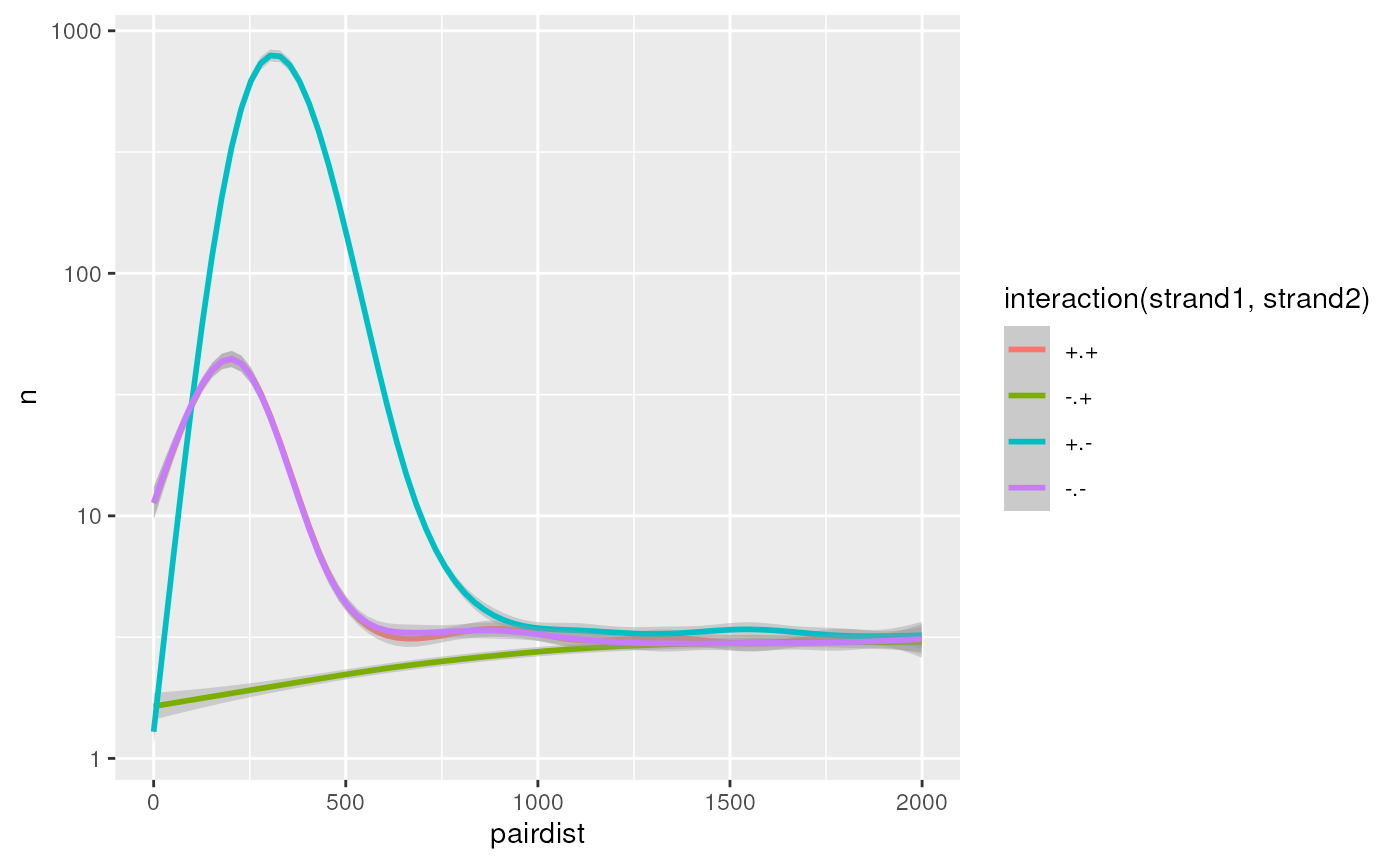

Plot P(s)

More generally, we can compute genome-wide genomic-distance-dependent interaction frequency, or P(s).

x <- 1.1^(1:200-1)
lmc <- coef(lm(c(1,1161443398)~c(x[1], x[200])))
bins_breaks <- unique(round(lmc[2]*x + lmc[1]))
bins_widths <- lead(bins_breaks) - bins_breaks

# Bin distances
df <- pairs |> 
    add_pairdist(colname = 's') |> 
    mutate(
        binned_s = bins_breaks[as.numeric(cut(s, bins_breaks))], 
        bin_width = bins_widths[as.numeric(cut(s, bins_breaks))]
    ) |> 
    group_by(binned_s, bin_width) |> 
    count(name = "n") |>
    as_tibble() |> 
    mutate(Ps = n / sum(n) / bin_width)

ggplot(df, aes(x = binned_s, y = Ps)) + 
    geom_line() + 
    scale_y_log10() +
    scale_x_log10() +
    annotation_logticks() + 
    labs(x = "Genomic distance", y = "Contact frequency") + 
    theme_bw()
#> Warning: Removed 1 row containing missing values or values outside the scale range
#> (`geom_line()`).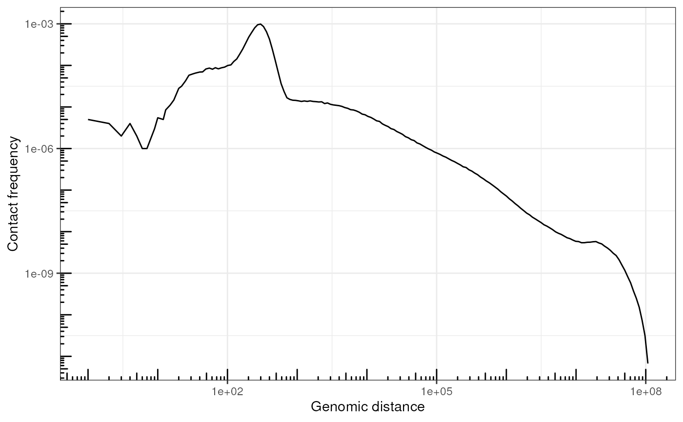

Manipulating coverage data

Introduction to `tidyCoverage`

`CoverageExperiment` and `AggregatedCoverage` class

Recommended time: 5 min

Both classes are built on top of SummarizedExperiment class of objects.

library(tidyCoverage)
#> 
#> Attaching package: 'tidyCoverage'
#> The following object is masked from 'package:S4Vectors':
#> 
#>     expand

data(ce)

data(ac)

ce
#> class: CoverageExperiment 
#> dim: 1 2 
#> metadata(0):
#> assays(1): coverage
#> rownames(1): Scc1
#> rowData names(2): features n
#> colnames(2): RNA_fwd RNA_rev
#> colData names(1): track
#> width: 3000

ac
#> class: AggregatedCoverage 
#> dim: 1 2 
#> metadata(0):
#> assays(8): mean median ... ci_low ci_high
#> rownames(1): Scc1
#> rowData names(1): features
#> colnames(2): RNA_fwd RNA_rev
#> colData names(1): track
#> width: 3000
#> binning: 1

Creating a `CoverageExperiment` object from tracks and features

Recommended time: 10 min

A CoverageExperiment object extracts coverage scores from tracks (typically a named BigWigFileList or a list of already imported RleLists), over a list of genomic ranges of interest (typically a named GRangesList).

tracks <- BigWigFileList(c(
    mnase = system.file("extdata", "MNase.bw", package = "tidyCoverage"), 
    cohesin = system.file("extdata", "Scc1.bw", package = "tidyCoverage")  
))
features <- GRangesList(
    TSSs = system.file("extdata", "TSSs.bed", package = "tidyCoverage") |> import() |> sample(2000), 
    TTSs = system.file("extdata", "TTSs.bed", package = "Bioc2024tidyWorkshop") |> import() |> sample(2000)
)

ce2 <- CoverageExperiment(
    tracks = tracks, 
    features = features,
    width = 2000, 
    ignore.strand = FALSE
)

ce2
#> class: CoverageExperiment 
#> dim: 2 2 
#> metadata(0):
#> assays(1): coverage
#> rownames(2): TSSs TTSs
#> rowData names(2): features n
#> colnames(2): mnase cohesin
#> colData names(1): track
#> width: 2000

Remember, this class of object is nearly identical to a SummarizedExperiment object.

The slight difference is that each cell of the coverage assay is a list with a single element which is an array.

colData(ce2)
#> DataFrame with 2 rows and 1 column
#>               track
#>         <character>
#> mnase         mnase
#> cohesin     cohesin

rowData(ce2)
#> DataFrame with 2 rows and 2 columns
#>         features         n
#>      <character> <integer>
#> TSSs        TSSs       553
#> TTSs        TTSs       537

assay(ce2, 'coverage')
#>      mnase           cohesin        
#> TSSs numeric,1106000 numeric,1106000
#> TTSs numeric,1074000 numeric,1074000

class(assay(ce2, 'coverage')['TSSs', 'mnase'])
#> [1] "list"

class(assay(ce2, 'coverage')[['TSSs', 'mnase']])
#> [1] "matrix" "array"

dim(assay(ce2, 'coverage')[['TSSs', 'mnase']])
#> [1]  553 2000

Tidy coverage? That’s right!

Recommended time: 5 min

Methods for tidyverse action verbs are available for CoverageExperiment objects, through the tidySummarizedExperiment package.

library(tidySummarizedExperiment)
#> Loading required package: ttservice
#> 
#> Attaching package: 'ttservice'
#> The following objects are masked from 'package:dplyr':
#> 
#>     bind_cols, bind_rows

ce2
#> # A CoverageExperiment-tibble abstraction: 4 × 7
#> # features=2 | tracks=2 | assays=coverage
#> # width=2000
#>   .feature .sample coverage            track   features     n GRangesList       
#>   <chr>    <chr>   <list>              <chr>   <chr>    <int> <list>            
#> 1 TSSs     mnase   <dbl [553 × 2,000]> mnase   TSSs       553 <tibble [553 × 8]>
#> 2 TTSs     mnase   <dbl [537 × 2,000]> mnase   TTSs       537 <tibble [537 × 8]>
#> 3 TSSs     cohesin <dbl [553 × 2,000]> cohesin TSSs       553 <tibble [553 × 8]>
#> 4 TTSs     cohesin <dbl [537 × 2,000]> cohesin TTSs       537 <tibble [537 × 8]>

ce2 |> filter(features == 'TSSs')
#> # A CoverageExperiment-tibble abstraction: 2 × 7
#> # features=1 | tracks=2 | assays=coverage
#> # width=2000
#>   .feature .sample coverage            track   features     n GRangesList       
#>   <chr>    <chr>   <list>              <chr>   <chr>    <int> <list>            
#> 1 TSSs     mnase   <dbl [553 × 2,000]> mnase   TSSs       553 <tibble [553 × 8]>
#> 2 TSSs     cohesin <dbl [553 × 2,000]> cohesin TSSs       553 <tibble [553 × 8]>

ce2 |> slice(2)
#> # A CoverageExperiment-tibble abstraction: 1 × 7
#> # features=1 | tracks=1 | assays=coverage
#> # width=2000
#>   .feature .sample coverage            track features     n GRangesList       
#>   <chr>    <chr>   <list>              <chr> <chr>    <int> <list>            
#> 1 TTSs     mnase   <dbl [537 × 2,000]> mnase TTSs       537 <tibble [537 × 8]>

ce2 |> select(features, n)
#> tidySummarizedExperiment says: Key columns are missing. A data frame is returned for independent data analysis.
#> # A tibble: 4 × 2
#>   features     n
#>   <chr>    <int>
#> 1 TSSs       553
#> 2 TTSs       537
#> 3 TSSs       553
#> 4 TTSs       537

`expand()` or `aggregate()`

Recommended time: 5 min

The expand method provided in the tidyCoverage package is used to turn a CoverageExperiment object into a tidy tibble.

tib <- expand(ce2)

tib
#> # A tibble: 4,360,000 × 8
#> # Groups:   track, features, ranges [2,180]
#>    track features chr   ranges             strand  coord coverage coord.scaled
#>    <chr> <fct>    <chr> <chr>              <chr>   <dbl>    <dbl>        <dbl>
#>  1 mnase TSSs     IV    IV:302211-304210:+ +      302211    0.936        -1000
#>  2 mnase TSSs     IV    IV:302211-304210:+ +      302212    0.936         -999
#>  3 mnase TSSs     IV    IV:302211-304210:+ +      302213    0.936         -998
#>  4 mnase TSSs     IV    IV:302211-304210:+ +      302214    0.936         -997
#>  5 mnase TSSs     IV    IV:302211-304210:+ +      302215    0.936         -996
#>  6 mnase TSSs     IV    IV:302211-304210:+ +      302216    0.936         -995
#>  7 mnase TSSs     IV    IV:302211-304210:+ +      302217    0.936         -994
#>  8 mnase TSSs     IV    IV:302211-304210:+ +      302218    0.936         -993
#>  9 mnase TSSs     IV    IV:302211-304210:+ +      302219    0.936         -992
#> 10 mnase TSSs     IV    IV:302211-304210:+ +      302220    0.936         -991
#> # ℹ 4,359,990 more rows

The aggregate method provided in the tidyCoverage package is used to turn a CoverageExperiment object into an AggregatedCoverage. This class of object stores different statistical measurements of the coverage over each element of the GRangesList provided in the CoverageExperiment object.

ac2 <- aggregate(ce2)

ac2
#> # An AggregatedCoverage-tibble abstraction: 8000 × 13
#> # features=2 | tracks=2 | assays=mean, median, min, max, sd, se, ci_low,
#> #   ci_high
#> # width=2000 | binning=1
#>    .sample .feature track features coord  mean median   min   max    sd     se
#>    <chr>   <fct>    <chr> <fct>    <dbl> <dbl>  <dbl> <dbl> <dbl> <dbl>  <dbl>
#>  1 mnase   TSSs     mnase TSSs     -1000  3.12   3.02     0  8.79  1.86 0.0789
#>  2 mnase   TSSs     mnase TSSs      -999  3.13   3.02     0  8.79  1.86 0.0790
#>  3 mnase   TSSs     mnase TSSs      -998  3.12   3.00     0  8.79  1.86 0.0791
#>  4 mnase   TSSs     mnase TSSs      -997  3.14   3.02     0  8.79  1.87 0.0794
#>  5 mnase   TSSs     mnase TSSs      -996  3.14   3.02     0  8.79  1.86 0.0791
#>  6 mnase   TSSs     mnase TSSs      -995  3.12   3.02     0  8.79  1.85 0.0787
#>  7 mnase   TSSs     mnase TSSs      -994  3.12   3.00     0  8.79  1.85 0.0786
#>  8 mnase   TSSs     mnase TSSs      -993  3.12   3.00     0  8.79  1.86 0.0789
#>  9 mnase   TSSs     mnase TSSs      -992  3.09   2.98     0  8.79  1.84 0.0783
#> 10 mnase   TSSs     mnase TSSs      -991  3.11   2.99     0  8.79  1.84 0.0783
#> # ℹ 7,990 more rows
#> # ℹ 2 more variables: ci_low <dbl>, ci_high <dbl>

Visualizing aggregated coverage

Recommended time: 10 min

The development version of tidyCoverage now ships two geom_* with appropriate default mapping aesthetics:

geom_coverage() for CoverageExperiment objects.
geom_aggrcoverage() for AggregatedCoverage objects.

CoverageExperiment(tracks, GRanges("II:1-100000"), window = 100) |>
    expand() |>
    ggplot() +
    geom_coverage() + 
    facet_grid(track ~ features, scales = "free") + 
    labs(x = 'chrV', y = 'Signal coverage')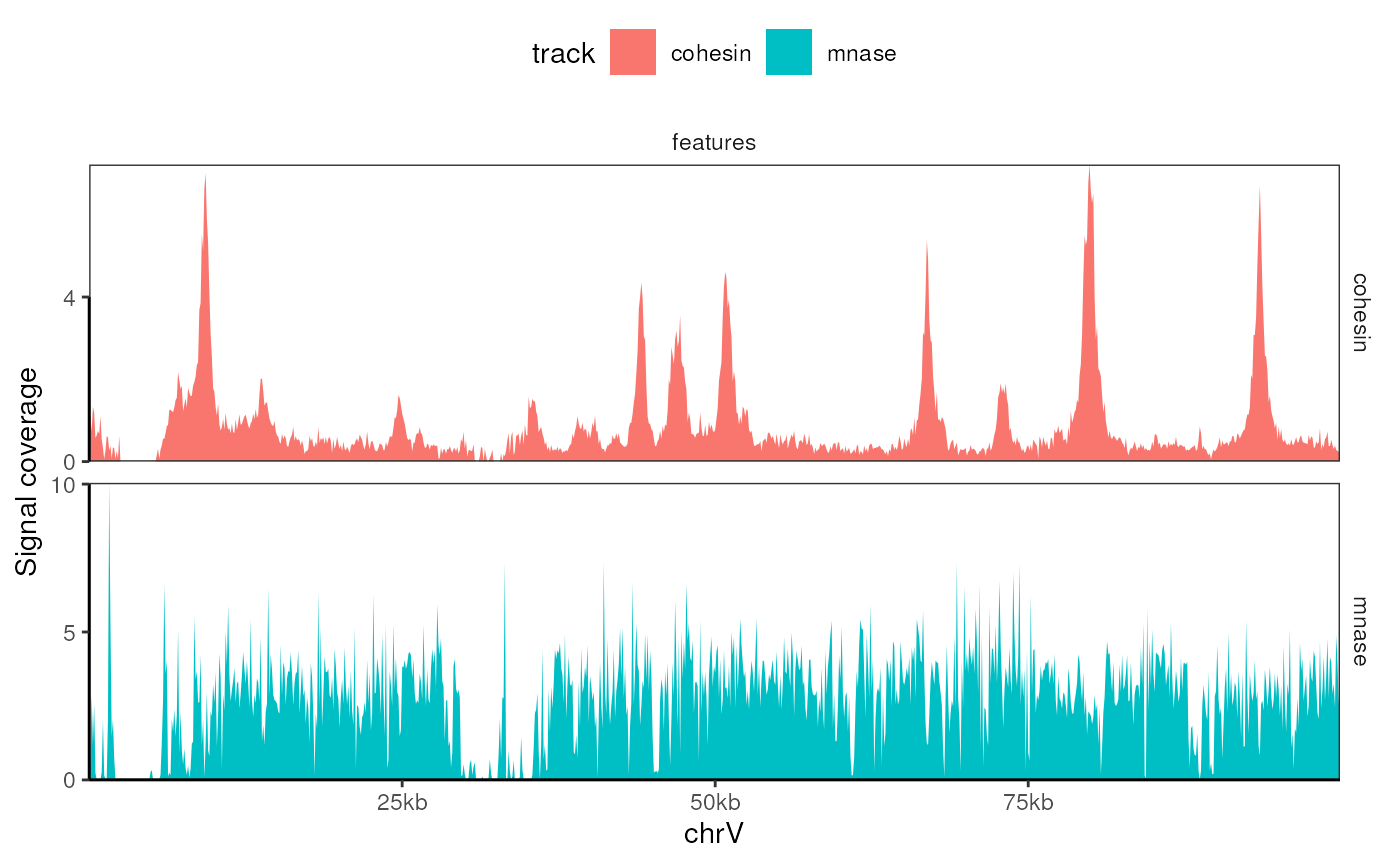


ggplot(ac2) + 
    geom_aggrcoverage() + 
    facet_grid(track ~ features, scales = "free") + 
    labs(x = 'Distance from genomic features', y = 'Signal coverage')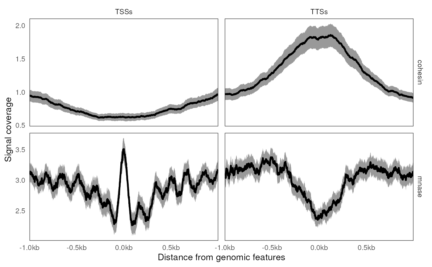

Real-world use case: studying epigenomic landscape of reulatory elements

Fetch coverage data from ENCODE

library(AnnotationHub)
#> Loading required package: BiocFileCache
#> Loading required package: dbplyr
#> 
#> Attaching package: 'dbplyr'
#> The following objects are masked from 'package:dplyr':
#> 
#>     ident, sql
#> 
#> Attaching package: 'AnnotationHub'
#> The following object is masked from 'package:Biobase':
#> 
#>     cache
#> The following object is masked from 'package:rtracklayer':
#> 
#>     hubUrl
ah <- AnnotationHub()
ids <- c('AH32207', 'AH35187')
names(ids) <- c('DNAse', 'H3K4me3')
bws <- lapply(ids, function(.x) ah[[.x]] |> resource()) |> BigWigFileList()
#> loading from cache
#> loading from cache
names(bws) <- names(ids)

Plotting coverage data over several loci

ce3 <- CoverageExperiment(
    bws, 
    list(
        ccno = GRanges("chr5:55220001-55235000"),
        mcidas = GRanges("chr5:55159001-55174000")
    ), 
    window = 50
)
expand(ce3) |> 
    mutate(coverage = scales::oob_squish(coverage, c(0, 10))) |> 
    ggplot() +
    geom_coverage(aes(fill = track), unit = 'Mb') + 
    facet_grid(track~features, scales = 'free')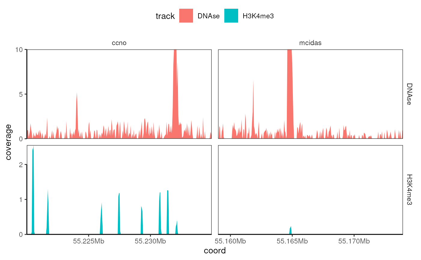

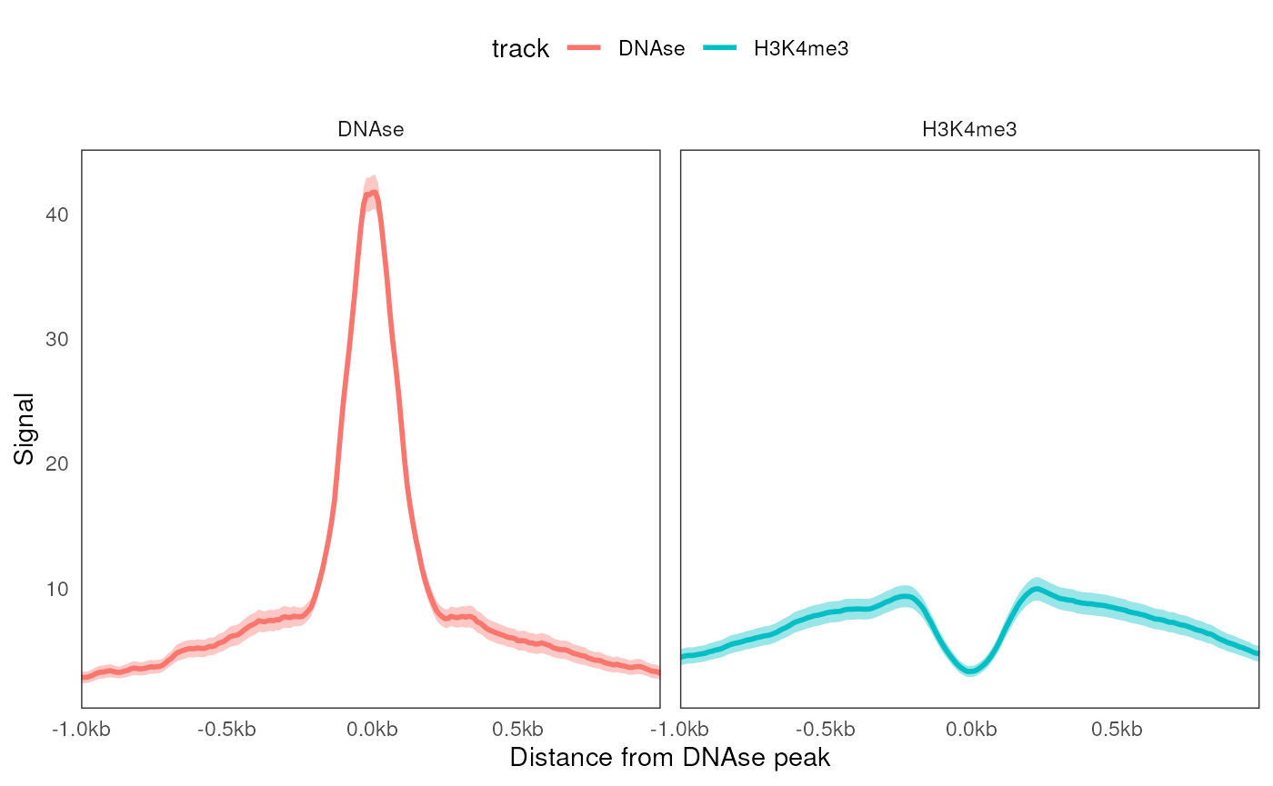
Import DNase peaks from ENCODE

features <- list(DNase = ah[['AH30077']] |> filter(zScore > 100) |> sample(1000))
#> loading from cache

Generating coverage aggregates and heatmaps over DNAse peak

ce4 <- CoverageExperiment(bws, features, width = 2000, window = 10)

aggregate(ce4) |> 
    ggplot(aes(x = coord, y = mean)) + 
    geom_aggrcoverage(aes(col = track)) + 
    facet_wrap(~track) + 
    labs(x = 'Distance from DNAse peak', y = 'Signal')

jacquesserizay@gmail.com,Institut Pasteur, Paris ↩︎

Jacques Serizay1

Manipulating genomic ranges data

Importing GRanges from files

Manipulating GRanges with tidy verbs

Manipulating genomic interaction data

What are GInteractions?

Creating a GInteractions object from scratch

Importing genomic interaction data from files

Manipulating GInteractions the tidy way

Moving anchors around

Filtering interactions

Overlapping anchors

Real-world use case: computing a P(s)

Importing data from pairs file

Counting interactions by strands

Plot P(s)

Manipulating coverage data

Introduction to tidyCoverage

CoverageExperiment and AggregatedCoverage class

Creating a CoverageExperiment object from tracks and features

Tidy coverage? That’s right!

expand() or aggregate()

Visualizing aggregated coverage

Real-world use case: studying epigenomic landscape of reulatory elements

Fetch coverage data from ENCODE

Plotting coverage data over several loci

Import DNase peaks from ENCODE

Generating coverage aggregates and heatmaps over DNAse peak

Jacques Serizay¹

Importing `GRanges` from files

Manipulating `GRanges` with tidy verbs

What are `GInteractions`?

Creating a `GInteractions` object from scratch

Manipulating `GInteractions` the tidy way

Introduction to `tidyCoverage`

`CoverageExperiment` and `AggregatedCoverage` class

Creating a `CoverageExperiment` object from tracks and features

`expand()` or `aggregate()`