# 15 Lab 8: Pseudotime analyses
> **NOTE:**
>
> The estimated time for this lab is around 1h30.
> **TIP:**
>
> - Perform pseudotime and lineage analysis
> - Model and visualize gene expression along pseudotime
> - Understand the requirements for RNA velocity computation
> - Compute RNA velocity and use it to orientate lineages
## 15.1 Process testis data in R
### 15.1.1 Import testis data from GSE112013 and pre-process it
We will work on a `testis` dataset, from the “The adult human testis transcriptional cell atlas” study ([Guo et al., Cell Research 2018](https://doi.org/10.1038/s41422-018-0099-2)). This dataset contains single-cell RNAseq data from human testis. It is available on the GEO database under the accession number [GSE112013](https://www.ncbi.nlm.nih.gov/geo/query/acc.cgi?acc=GSE112013).
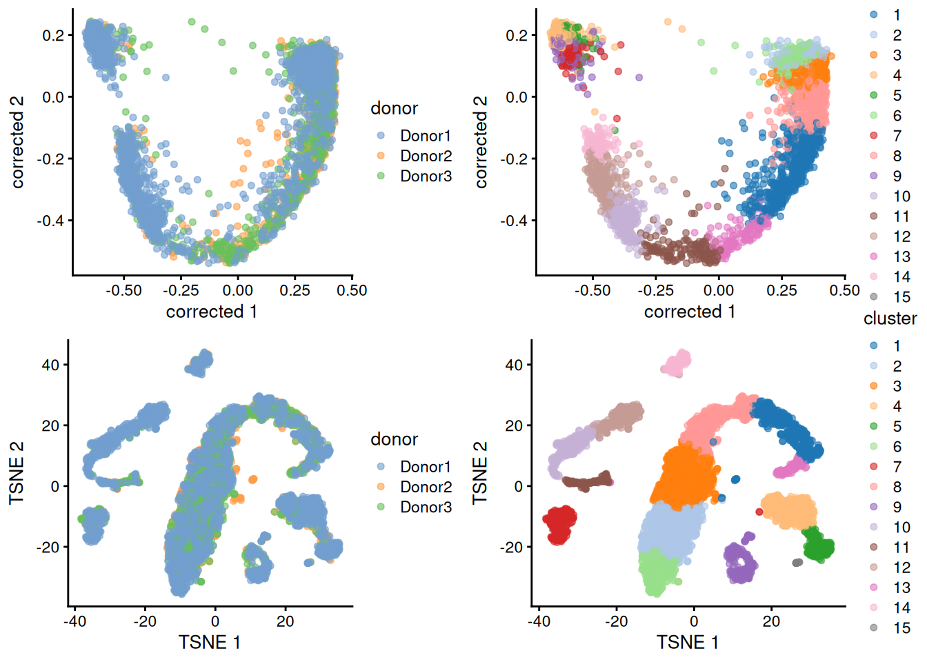
We have applied the different analysis steps we have learned over the past three days to the count matrix `GSE112013_Combined_UMI_table.txt.gz`. See the code below for the details of pre-processing steps, and run it in your session (this takes a few minutes, and requires ~8 GB of memory).
> **NOTE:**
>
> Check the GEO page for supplementary processed data, and download the `GSE112013_Combined_UMI_table.txt.gz` table.
>
> With this data, we will:
>
> - Import the dataset in R as a `SingleCellExperiment` object,
> - Remove doublets,
> - Filter genes and cells,
> - Normalize `counts`,
> - Correct for batch effect,
> - Cluster cells.
>
> ``` r
> library(SingleCellExperiment)
> ## Loading required package: SummarizedExperiment
> ## Loading required package: MatrixGenerics
> ## Loading required package: matrixStats
> ##
> ## Attaching package: 'MatrixGenerics'
> ## The following objects are masked from 'package:matrixStats':
> ##
> ## colAlls, colAnyNAs, colAnys, colAvgsPerRowSet, colCollapse,
> ## colCounts, colCummaxs, colCummins, colCumprods, colCumsums,
> ## colDiffs, colIQRDiffs, colIQRs, colLogSumExps, colMadDiffs,
> ## colMads, colMaxs, colMeans2, colMedians, colMins, colOrderStats,
> ## colProds, colQuantiles, colRanges, colRanks, colSdDiffs, colSds,
> ## colSums2, colTabulates, colVarDiffs, colVars, colWeightedMads,
> ## colWeightedMeans, colWeightedMedians, colWeightedSds,
> ## colWeightedVars, rowAlls, rowAnyNAs, rowAnys, rowAvgsPerColSet,
> ## rowCollapse, rowCounts, rowCummaxs, rowCummins, rowCumprods,
> ## rowCumsums, rowDiffs, rowIQRDiffs, rowIQRs, rowLogSumExps,
> ## rowMadDiffs, rowMads, rowMaxs, rowMeans2, rowMedians, rowMins,
> ## rowOrderStats, rowProds, rowQuantiles, rowRanges, rowRanks,
> ## rowSdDiffs, rowSds, rowSums2, rowTabulates, rowVarDiffs,
> ## rowVars, rowWeightedMads, rowWeightedMeans, rowWeightedMedians,
> ## rowWeightedSds, rowWeightedVars
> ## Loading required package: GenomicRanges
> ## Loading required package: stats4
> ## Loading required package: BiocGenerics
> ## Loading required package: generics
> ##
> ## Attaching package: 'generics'
> ## The following objects are masked from 'package:base':
> ##
> ## as.difftime, as.factor, as.ordered, intersect, is.element,
> ## setdiff, setequal, union
> ##
> ## Attaching package: 'BiocGenerics'
> ## The following objects are masked from 'package:stats':
> ##
> ## IQR, mad, sd, var, xtabs
> ## The following object is masked from 'package:utils':
> ##
> ## data
> ## The following objects are masked from 'package:base':
> ##
> ## Filter, Find, Map, Position, Reduce, anyDuplicated, aperm,
> ## append, as.data.frame, basename, cbind, colnames, dirname,
> ## do.call, duplicated, eval, evalq, get, grep, grepl, is.unsorted,
> ## lapply, mapply, match, mget, order, paste, pmax, pmax.int, pmin,
> ## pmin.int, rank, rbind, rownames, sapply, saveRDS, scale,
> ## sequence, table, tapply, transform, unique, unsplit, which.max,
> ## which.min
> ## Loading required package: S4Vectors
> ##
> ## Attaching package: 'S4Vectors'
> ## The following object is masked from 'package:utils':
> ##
> ## findMatches
> ## The following objects are masked from 'package:base':
> ##
> ## I, expand.grid, unname
> ## Loading required package: IRanges
> ## Loading required package: Seqinfo
> ## Loading required package: Biobase
> ## Welcome to Bioconductor
> ##
> ## Vignettes contain introductory material; view with
> ## 'browseVignettes()'. To cite Bioconductor, see
> ## 'citation("Biobase")', and for packages 'citation("pkgname")'.
> ##
> ## Attaching package: 'Biobase'
> ## The following object is masked from 'package:MatrixGenerics':
> ##
> ## rowMedians
> ## The following objects are masked from 'package:matrixStats':
> ##
> ## anyMissing, rowMedians
> library(tidyverse)
> ## ── Attaching core tidyverse packages ───────────────────── tidyverse 2.0.0 ──
> ## ✔ dplyr 1.2.1 ✔ readr 2.2.0
> ## ✔ forcats 1.0.1 ✔ stringr 1.6.0
> ## ✔ ggplot2 4.0.3 ✔ tibble 3.3.1
> ## ✔ lubridate 1.9.5 ✔ tidyr 1.3.2
> ## ✔ purrr 1.2.2
> ## ── Conflicts ─────────────────────────────────────── tidyverse_conflicts() ──
> ## ✖ lubridate::%within%() masks IRanges::%within%()
> ## ✖ ggplot2::Position() masks BiocGenerics::Position(), base::Position()
> ## ✖ dplyr::collapse() masks IRanges::collapse()
> ## ✖ dplyr::combine() masks Biobase::combine(), BiocGenerics::combine()
> ## ✖ dplyr::count() masks matrixStats::count()
> ## ✖ dplyr::desc() masks IRanges::desc()
> ## ✖ tidyr::expand() masks S4Vectors::expand()
> ## ✖ dplyr::filter() masks stats::filter()
> ## ✖ dplyr::first() masks S4Vectors::first()
> ## ✖ dplyr::lag() masks stats::lag()
> ## ✖ purrr::reduce() masks GenomicRanges::reduce(), IRanges::reduce()
> ## ✖ dplyr::rename() masks S4Vectors::rename()
> ## ✖ lubridate::second() masks S4Vectors::second()
> ## ✖ lubridate::second<-() masks S4Vectors::second<-()
> ## ✖ dplyr::slice() masks IRanges::slice()
> ## ℹ Use the conflicted package () to force all conflicts to become errors
>
> # Download raw file
> library(BiocFileCache)
> ## Loading required package: dbplyr
> ##
> ## Attaching package: 'dbplyr'
> ##
> ## The following objects are masked from 'package:dplyr':
> ##
> ## ident, sql, sql_escape_ident, sql_escape_string
> ##
> ## OpenTelemetry error: there is no package called 'otelsdk'
> ## OpenTelemetry error: there is no package called 'otelsdk'
> bfc <- BiocFileCache(ask = FALSE)
> umi_file <- bfcrpath(bfc, 'https://ftp.ncbi.nlm.nih.gov/geo/series/GSE112nnn/GSE112013/suppl/GSE112013_Combined_UMI_table.txt.gz')
> ## adding rname 'https://ftp.ncbi.nlm.nih.gov/geo/series/GSE112nnn/GSE112013/suppl/GSE112013_Combined_UMI_table.txt.gz'
>
> # Create SingleCellExperiment object
> x <- data.table::fread(umi_file, data.table = FALSE)
> counts <- as(as.matrix(x[, -1]), 'dgCMatrix')
> rownames(counts) <- x[, 1]
> rm(x); invisible(gc())
> testis <- SingleCellExperiment(
> assays = list(counts = counts),
> colData = DataFrame(cellid = colnames(counts))
> )
> testis$Barcode <- str_replace(testis$cellid, 'Donor.-', '') |> str_replace('-.', '')
> testis$donor <- str_replace(testis$cellid, '-.*', '')
> testis$replicate <- str_replace(testis$cellid, '.*-', '')
> testis$sample <- paste0(testis$donor, '_rep', testis$replicate)
> table(testis$donor, testis$replicate)
> ##
> ## 1 2
> ## Donor1 1000 1248
> ## Donor2 985 1009
> ## Donor3 1116 1132
>
> # Remove doublets
> set.seed(1000)
> testis <- scDblFinder::scDblFinder(testis, samples = testis$sample)
> ##
> |
> | | 0%
> |
> |=========== | 17%
> |
> |====================== | 33%
> |
> |================================== | 50%
> |
> |============================================= | 67%
> |
> |======================================================== | 83%
> |
> |===================================================================| 100%
> table(testis$scDblFinder.class)
> ##
> ## singlet doublet
> ## 6224 266
> testis <- testis[, testis$scDblFinder.class == 'singlet']
>
> # Recover Ensembl IDs and biotypes for genes, and keep protein-coding genes
> gene_info <- AnnotationDbi::select(
> org.Hs.eg.db::org.Hs.eg.db,
> keys = rownames(testis), keytype = 'SYMBOL',
> columns = c('ENSEMBL', 'GENETYPE')
> ) |>
> filter(GENETYPE == 'protein-coding') |>
> distinct(SYMBOL, .keep_all = TRUE)
> ##
> ## 'select()' returned 1:many mapping between keys and columns
> testis <- testis[gene_info$SYMBOL, ]
> rowData(testis)$gene_name <- gene_info$SYMBOL
> rowData(testis)$gene_id <- gene_info$ENSEMBL
>
> # Get QCs per cell, flag low-quality cells and filter them out
> mito <- grep('^MT-', rownames(testis), value = TRUE)
> testis <- scrapper::quickRnaQc.se(testis, subsets = list(mito = mito), block = testis$sample)
> table(testis$keep)
> ##
> ## FALSE TRUE
> ## 832 5392
> testis <- testis[, testis$keep]
>
> # Filter out genes not expressed in at least 10 cells
> testis <- testis[Matrix::rowSums(counts(testis) > 0) >= 10, ]
>
> # Normalize counts
> clusters <- scran::quickCluster(testis, block = testis$sample)
> testis <- scran::computeSumFactors(testis, clusters = clusters)
> testis <- scrapper::normalizeRnaCounts.se(
> testis, size.factors = sizeFactors(testis), block = testis$sample,
> more.norm.args = list(delayed = FALSE)
> )
>
> # Computing biological variance of each gene
> testis <- scrapper::chooseRnaHvgs.se(testis, block = testis$donor, top = 2000)
> rowData(testis)$isHVG <- rowData(testis)$hvg
> HVGs <- rownames(testis)[rowData(testis)$isHVG]
>
> # Embedding dataset in PCA space, correcting for batch effect
> mergedBatches <- batchelor::fastMNN(
> testis,
> batch = testis$donor,
> subset.row = HVGs
> )
> reducedDim(testis, 'corrected') <- reducedDim(mergedBatches, 'corrected')
>
> # Cluster cells using shared nearest-neighbors graph and Louvain community finding algorithm
> testis <- scrapper::clusterGraph.se(testis, reddim.type = 'corrected', output.name = 'cluster')
> testis$cluster <- factor(testis$cluster)
> table(testis$cluster)
> ##
> ## 1 2 3 4 5 6 7 8 9 10 11 12 13 14 15
> ## 519 754 806 471 241 347 288 534 302 335 176 304 128 168 19
>
> # Embedding dataset in TSNE space for visualization
> set.seed(10)
> testis <- scater::runTSNE(testis, dimred = 'corrected')
>
> # Visualize embeddings
> p <- cowplot::plot_grid(
> scater::plotReducedDim(testis, 'corrected', colour_by = 'donor'),
> scater::plotReducedDim(testis, 'corrected', colour_by = 'cluster'),
> scater::plotReducedDim(testis, 'TSNE', colour_by = 'donor'),
> scater::plotReducedDim(testis, 'TSNE', colour_by = 'cluster')
> )
> p
> ```
>
> 
### 15.1.2 Annotate cells using HPA resources
The [Human Protein Atlas (HPA)](https://www.proteinatlas.org) is a valuable resource for cell type annotations. It provides single-cell RNAseq data for a large number of cell types.
> **NOTE:**
>
> Download `HPA` scRNAseq atlas (combined per cell type) [from here](https://www.proteinatlas.org/download/tsv/rna_single_cell_type.tsv.zip), and import it in R as a `SummarizedExperiment` object.
>
> > **NOTE:**
> >
> > ``` r
> > hpa_file <- bfcrpath(bfc, 'https://www.proteinatlas.org/download/tsv/rna_single_cell_type.tsv.zip')
> > ## adding rname 'https://www.proteinatlas.org/download/tsv/rna_single_cell_type.tsv.zip'
> > HPA <- read_tsv(hpa_file) |>
> > dplyr::select(-Gene) |>
> > pivot_wider(names_from = `Cell type`, values_from = 'nCPM', values_fn = mean) |>
> > distinct(`Gene name`, .keep_all = TRUE) |>
> > column_to_rownames('Gene name') |>
> > as.matrix()
> > ## Rows: 3107242 Columns: 4
> > ## ── Column specification ─────────────────────────────────────────────────────
> > ## Delimiter: "\t"
> > ## chr (3): Gene, Gene name, Cell type
> > ## dbl (1): nCPM
> > ##
> > ## ℹ Use `spec()` to retrieve the full column specification for this data.
> > ## ℹ Specify the column types or set `show_col_types = FALSE` to quiet this message.
> > HPA[is.na(HPA)] <- 0
> > HPA_se <- SummarizedExperiment::SummarizedExperiment(
> > assays = list('logcounts' = log2(HPA + 1)),
> > colData = DataFrame(cell_type = colnames(HPA))
> > )
> > HPA_se
> > ## class: SummarizedExperiment
> > ## dim: 20151 155
> > ## metadata(0):
> > ## assays(1): logcounts
> > ## rownames(20151): TSPAN6 TNMD ... ENSG00000291316 TMEM276
> > ## rowData names(0):
> > ## colnames(155): adipocytes adrenal cortex cells ... vascular
> > ## endothelial cells vascular smooth muscle cells
> > ## colData names(1): cell_type
> > ```
>
> How many and what cell types are profiled?
>
> > **NOTE:**
> >
> > ``` r
> > length(HPA_se$cell_type)
> > ## [1] 155
> > HPA_se$cell_type
> > ## [1] "adipocytes"
> > ## [2] "adrenal cortex cells"
> > ## [3] "adrenal medulla cells"
> > ## [4] "alveolar cells type 1"
> > ## [5] "alveolar cells type 2"
> > ## [6] "astrocytes"
> > ## [7] "b-cells"
> > ## [8] "basal keratinocytes"
> > ## [9] "basal prostatic cells"
> > ## [10] "basophils"
> > ## [11] "bergmann glia"
> > ## [12] "bone marrow mscs"
> > ## [13] "brain excitatory neurons"
> > ## [14] "brain inhibitory neurons"
> > ## [15] "breast hormone-responsive cells"
> > ## [16] "breast lactating cells"
> > ## [17] "breast myoepithelial cells"
> > ## [18] "breast secretory cells"
> > ## [19] "cardiomyocytes"
> > ## [20] "cdcs"
> > ## [21] "cholangiocytes"
> > ## [22] "choroid plexus epithelial cells"
> > ## [23] "colonocytes"
> > ## [24] "cone photoreceptor cells"
> > ## [25] "conjunctival goblet cells"
> > ## [26] "corticotrophs"
> > ## [27] "cytotrophoblasts"
> > ## [28] "decidual stromal cells"
> > ## [29] "differentiating spermatogonia"
> > ## [30] "distal convoluted tubule cells"
> > ## [31] "early primary spermatocytes"
> > ## [32] "early spermatids"
> > ## [33] "endometrial ciliated cells"
> > ## [34] "endometrial glandular cells"
> > ## [35] "endometrial luminal cells"
> > ## [36] "endometrial secretory cells"
> > ## [37] "endometrial stromal cells"
> > ## [38] "enteric stem cells"
> > ## [39] "enteric transient amplifying cells"
> > ## [40] "enterocytes"
> > ## [41] "enteroendocrine cells"
> > ## [42] "ependymal cells"
> > ## [43] "epididymal basal cells"
> > ## [44] "epididymal clear cells"
> > ## [45] "epididymal efferent duct absorptive cells"
> > ## [46] "epididymal efferent duct ciliated cells"
> > ## [47] "epididymal principal cells"
> > ## [48] "erythrocyte progenitors"
> > ## [49] "erythrocytes"
> > ## [50] "esophageal apical cells"
> > ## [51] "esophageal basal cells"
> > ## [52] "esophageal suprabasal cells"
> > ## [53] "extravillous trophoblasts"
> > ## [54] "fallopian secretory cells"
> > ## [55] "fallopian tube ciliated cells"
> > ## [56] "fibro-adipogenic progenitors"
> > ## [57] "fibroblasts"
> > ## [58] "foveolar cells"
> > ## [59] "gastric chief cells"
> > ## [60] "gastric progenitor cells"
> > ## [61] "goblet cells"
> > ## [62] "gonadotrophs"
> > ## [63] "granulosa cells"
> > ## [64] "hematopoietic stem cells"
> > ## [65] "hepatic stellate cells"
> > ## [66] "hepatocytes"
> > ## [67] "hofbauer cells"
> > ## [68] "innate lymphoid cells"
> > ## [69] "kupffer cells"
> > ## [70] "lacrimal acinar cells"
> > ## [71] "lactotrophs"
> > ## [72] "late primary spermatocytes"
> > ## [73] "late spermatids"
> > ## [74] "leydig cells"
> > ## [75] "loop of henle epithelial cells"
> > ## [76] "lymphatic endothelial cells"
> > ## [77] "macrophages"
> > ## [78] "mast cells"
> > ## [79] "medullary thymic epithelial cells"
> > ## [80] "megakaryocyte progenitors"
> > ## [81] "megakaryocyte-erythroid progenitors"
> > ## [82] "megakaryocytes"
> > ## [83] "melanocytes"
> > ## [84] "mesothelial cells"
> > ## [85] "microglia"
> > ## [86] "migrating cytotrophoblasts"
> > ## [87] "monocyte progenitors"
> > ## [88] "monocytes"
> > ## [89] "mucous neck cells"
> > ## [90] "müller glia"
> > ## [91] "myonuclei"
> > ## [92] "myosatellite cells"
> > ## [93] "neutrophil progenitors"
> > ## [94] "neutrophils"
> > ## [95] "nk-cells"
> > ## [96] "ocular epithelial cells"
> > ## [97] "oligodendrocyte progenitor cells"
> > ## [98] "oligodendrocytes"
> > ## [99] "oocytes"
> > ## [100] "other brain neurons"
> > ## [101] "ovarian stromal cells"
> > ## [102] "pancreatic acinar cells"
> > ## [103] "pancreatic duct cells"
> > ## [104] "pancreatic islet cells"
> > ## [105] "paneth cells"
> > ## [106] "papillary tip epithelial cells"
> > ## [107] "parietal cells"
> > ## [108] "pdcs"
> > ## [109] "pericytes"
> > ## [110] "peritubular myoid cells"
> > ## [111] "pituicytes/fscs"
> > ## [112] "pituitary stem cells"
> > ## [113] "plasma cells"
> > ## [114] "platelets"
> > ## [115] "podocytes"
> > ## [116] "prostatic club cells"
> > ## [117] "prostatic glandular cells"
> > ## [118] "prostatic hillock cells"
> > ## [119] "proximal tubule cells"
> > ## [120] "renal collecting duct intercalated cells"
> > ## [121] "renal collecting duct principal cells"
> > ## [122] "renal connecting tubule cells"
> > ## [123] "respiratory basal cells"
> > ## [124] "respiratory ciliated cells"
> > ## [125] "respiratory deuterosomal cells"
> > ## [126] "respiratory ionocytes"
> > ## [127] "respiratory secretory cells"
> > ## [128] "retinal amacrine cells"
> > ## [129] "retinal bipolar cells"
> > ## [130] "retinal ganglion cells"
> > ## [131] "retinal horizontal cells"
> > ## [132] "retinal pigment epithelial cells"
> > ## [133] "rod photoreceptor cells"
> > ## [134] "salivary acinar cells"
> > ## [135] "salivary basal cells"
> > ## [136] "salivary duct cells"
> > ## [137] "salivary ionocytes"
> > ## [138] "salivary myoepithelial cells"
> > ## [139] "schwann cells"
> > ## [140] "sertoli cells"
> > ## [141] "smooth muscle cells"
> > ## [142] "somatotrophs"
> > ## [143] "submucosal glandular cells"
> > ## [144] "suprabasal keratinocytes"
> > ## [145] "syncytiotrophoblasts"
> > ## [146] "t-cells"
> > ## [147] "thymic myoid cells"
> > ## [148] "thymocytes"
> > ## [149] "thyrotrophs"
> > ## [150] "transitional alveolar cells"
> > ## [151] "tuft cells"
> > ## [152] "undifferentiated spermatogonia"
> > ## [153] "urothelial cells"
> > ## [154] "vascular endothelial cells"
> > ## [155] "vascular smooth muscle cells"
> > ```
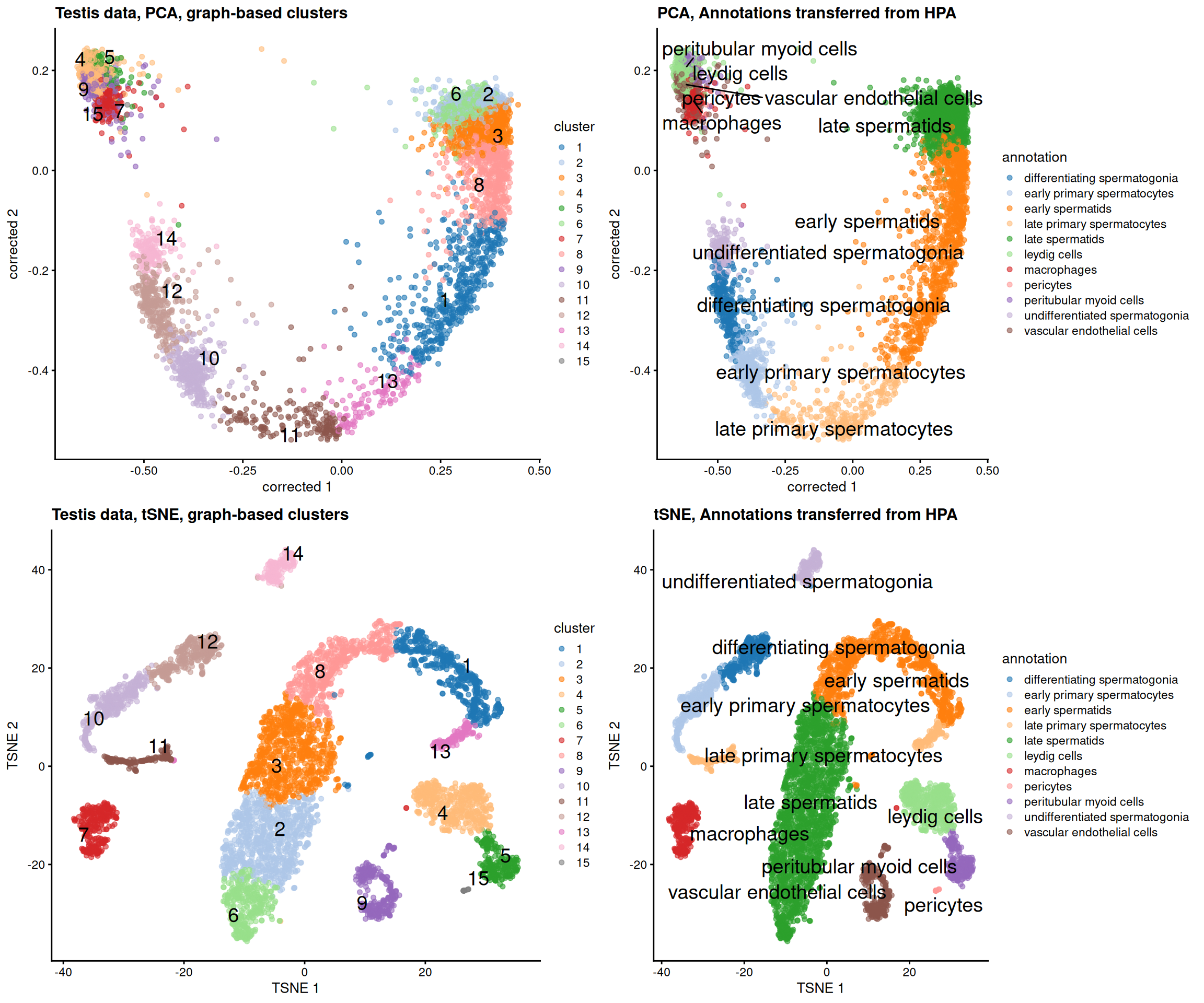
We can use the HPA reference to annotate cell types in the testis dataset.
> **NOTE:**
>
> Use `SingleR` to annotate cell types in the testis dataset using HPA reference.
>
> > **NOTE:**
> >
> > ``` r
> > predictions <- SingleR::SingleR(
> > test = testis,
> > ref = HPA_se,
> > labels = colData(HPA_se)$cell_type,
> > clusters = testis$cluster
> > )
> > testis$annotation <- predictions$labels[testis$cluster]
> > table(testis$annotation)
> > ##
> > ## differentiating spermatogonia early primary spermatocytes
> > ## 304 335
> > ## early spermatids late primary spermatocytes
> > ## 1053 304
> > ## late spermatids leydig cells
> > ## 1907 471
> > ## macrophages pericytes
> > ## 288 19
> > ## peritubular myoid cells undifferentiated spermatogonia
> > ## 241 168
> > ## vascular endothelial cells
> > ## 302
> > cowplot::plot_grid(
> > scater::plotReducedDim(testis, dimred = 'corrected', colour_by = 'cluster', text_by = 'cluster') + ggtitle('Testis data, PCA, graph-based clusters'),
> > scater::plotReducedDim(testis, dimred = 'corrected', colour_by = 'annotation', text_by = 'annotation') + ggtitle('PCA, Annotations transferred from HPA'),
> > scater::plotReducedDim(testis, dimred = 'TSNE', colour_by = 'cluster', text_by = 'cluster') + ggtitle('Testis data, tSNE, graph-based clusters'),
> > scater::plotReducedDim(testis, dimred = 'TSNE', colour_by = 'annotation', text_by = 'annotation') + ggtitle('tSNE, Annotations transferred from HPA')
> > )
> > ```
> >
> > 
### 15.1.3 Filter the testis dataset to only germinal cells.
In this notebook, we will focus on germinal cells only.
> **NOTE:**
>
> Filter the `testis` dataset to only retain germinal cells.
>
> > **NOTE:**
> >
> > ``` r
> > germcell_types <- c(
> > "undifferentiated spermatogonia", "differentiating spermatogonia",
> > "early primary spermatocytes", "late primary spermatocytes",
> > "early spermatids", "late spermatids"
> > )
> > germcells <- testis[, testis$annotation %in% germcell_types]
> > germcells$annotation <- factor(germcells$annotation, levels = intersect(germcell_types, germcells$annotation))
> > table(germcells$annotation)
> > ##
> > ## undifferentiated spermatogonia differentiating spermatogonia
> > ## 168 304
> > ## early primary spermatocytes late primary spermatocytes
> > ## 335 304
> > ## early spermatids late spermatids
> > ## 1053 1907
> > ```
## 15.2 Trajectory inference (TI) in scRNAseq
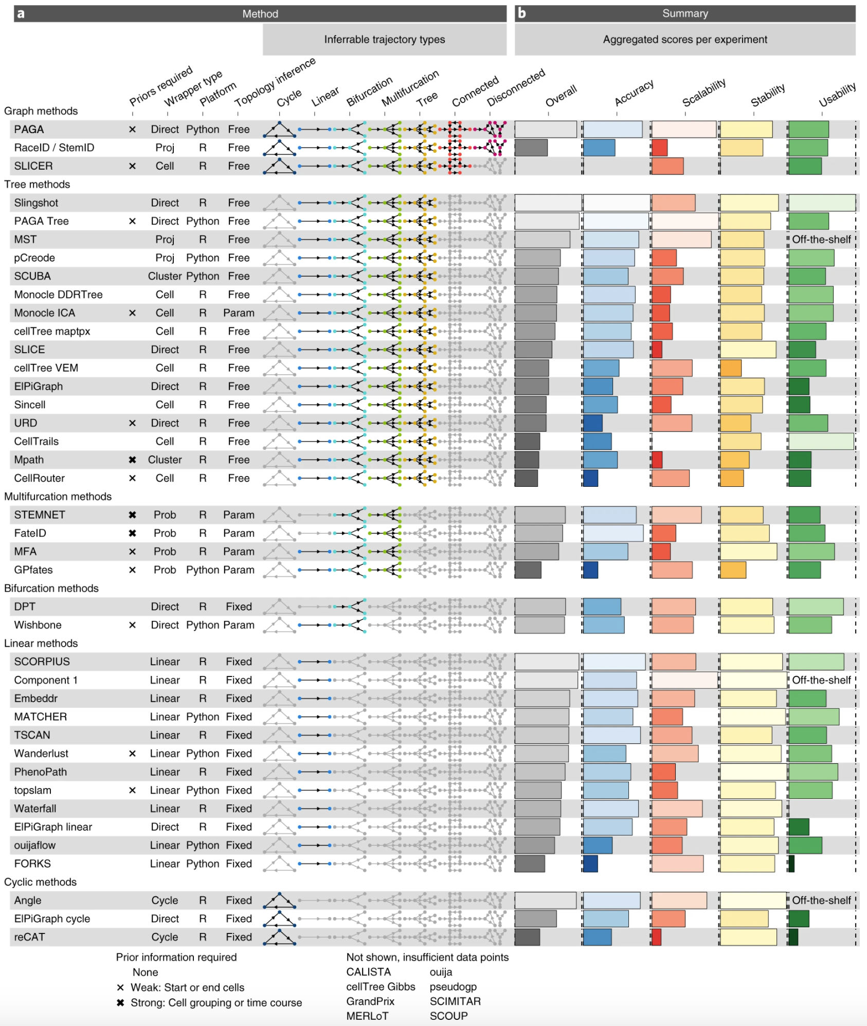
An important question in scRNAseq field of research is: how to identify a cell trajectory from high-dimensional expression data and map individual cells onto it? A large number of methods have currently emerged, each one with their own specificities, assumptions, and strengths. A nice breakdown (from 2019, so already very outdated!) is available from `Saelens et al., Nat. Biotech. 2019` (doi: 10.1038/s41587-019-0071-9):
### 15.2.1 Trajectory
`Slingshot` is perhaps one of the most widely used algorithms for users who want to focus on `R`-based approaches.
> **NOTE:**
>
> Read Slingshot documentation to understand how to identify lineages in a scRNAseq dataset in R.
>
> Why is it recommended to infer lineages from PCA space rather than t-SNE or UMAP space, even though these spaces do “reveal” an obvious trajectory in 2D?
>
> Infer lineages, using cluster annotations as information to build the MST. Note that you will first need to remove the 50th dimension of the `corrected` embedding for `slingshot` to work ([bug reported](https://github.com/kstreet13/slingshot/issues/87)).
>
> > **NOTE:**
> >
> > ``` r
> > reducedDim(germcells, 'corrected_2') <- reducedDim(germcells, 'corrected')[, 1:49]
> > germcells_slingshot <- slingshot::slingshot(
> > germcells,
> > reducedDim = 'corrected_2',
> > clusterLabels = germcells$annotation
> > )
> > slingshot::slingLineages(germcells_slingshot)
> > ## $Lineage1
> > ## [1] "late spermatids" "early spermatids"
> > ## [3] "late primary spermatocytes" "early primary spermatocytes"
> > ## [5] "differentiating spermatogonia" "undifferentiated spermatogonia"
> > ```
### 15.2.2 Pseudotime
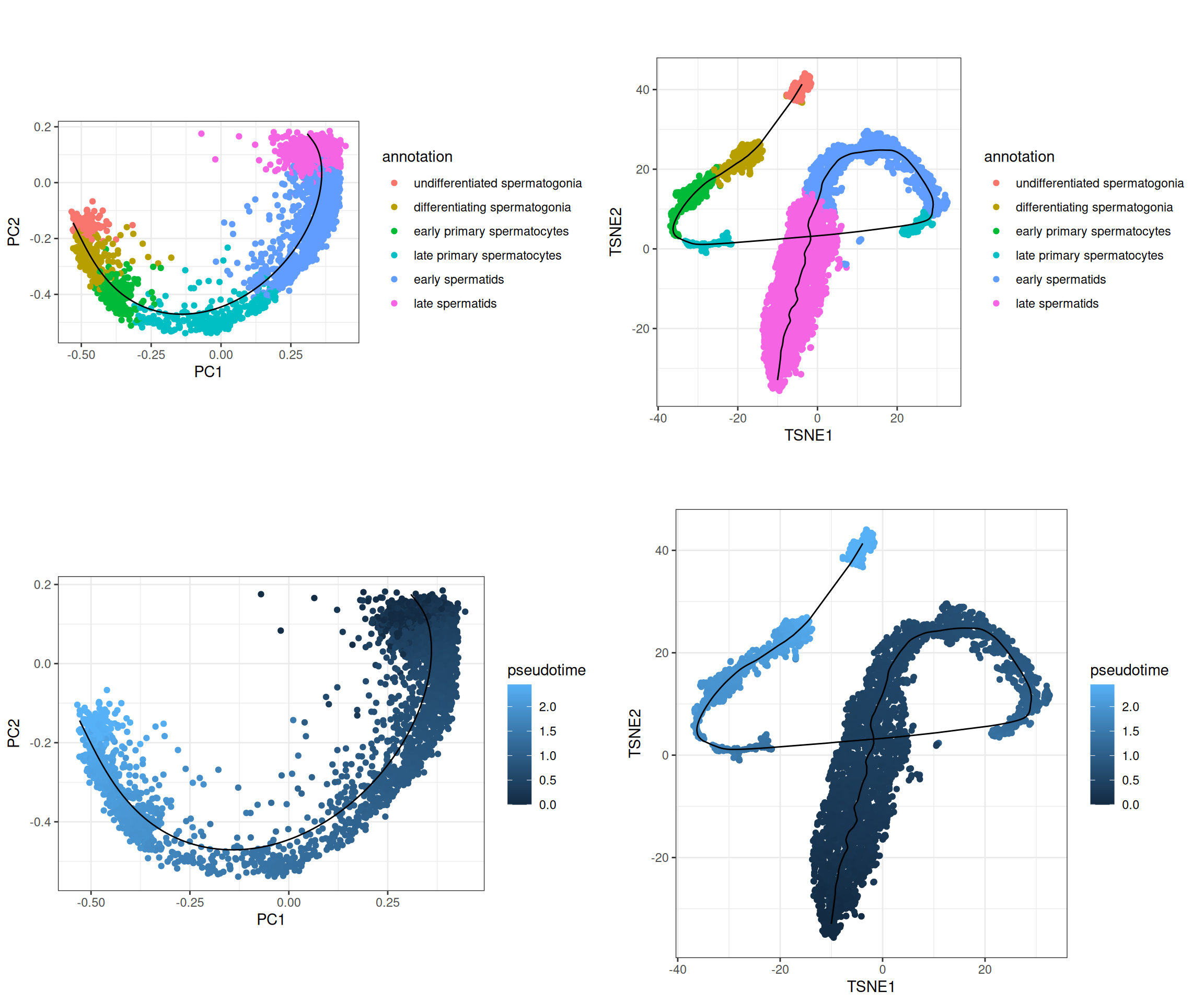
`slingshot` automatically deduces a pseudotime for each cell, based on the inferred lineage. It can be useful to visualize the trajectory of cells in a 2D space, and to order cells along the trajectory.
> **NOTE:**
>
> Recover pseudotime values and principal curves from `slingshot` output.
>
> > **NOTE:**
> >
> > ``` r
> > # Fetching pseudotime
> > germcells$pseudotime <- slingshot::slingPseudotime(germcells_slingshot)[, 'Lineage1']
> >
> > # Fetching principal curve in PCA space
> > pca_curve <- slingshot::slingCurves(germcells_slingshot, as.df = TRUE)
> > colnames(pca_curve)
> > ## [1] "Dim.1" "Dim.2" "Dim.3" "Dim.4" "Dim.5" "Dim.6" "Dim.7"
> > ## [8] "Dim.8" "Dim.9" "Dim.10" "Dim.11" "Dim.12" "Dim.13" "Dim.14"
> > ## [15] "Dim.15" "Dim.16" "Dim.17" "Dim.18" "Dim.19" "Dim.20" "Dim.21"
> > ## [22] "Dim.22" "Dim.23" "Dim.24" "Dim.25" "Dim.26" "Dim.27" "Dim.28"
> > ## [29] "Dim.29" "Dim.30" "Dim.31" "Dim.32" "Dim.33" "Dim.34" "Dim.35"
> > ## [36] "Dim.36" "Dim.37" "Dim.38" "Dim.39" "Dim.40" "Dim.41" "Dim.42"
> > ## [43] "Dim.43" "Dim.44" "Dim.45" "Dim.46" "Dim.47" "Dim.48" "Dim.49"
> > ## [50] "Order" "Lineage"
> > ## Rename the coordinates columns (all but the last two, `Order` and `Lineage`)
> > ndims <- ncol(pca_curve) - 2
> > colnames(pca_curve)[seq_len(ndims)] <- paste0('PC', seq_len(ndims))
> > head(pca_curve[, c('PC1', 'PC2', 'Order', 'Lineage')])
> > ## PC1 PC2 Order Lineage
> > ## 1 0.3085413 0.1750947 1 1
> > ## 2 0.3106834 0.1724270 2 1
> > ## 3 0.3128256 0.1697593 3 1
> > ## 4 0.3149677 0.1670916 4 1
> > ## 5 0.3171095 0.1644158 5 1
> > ## 6 0.3192504 0.1617224 6 1
> > ```
>
> We would like to visualize the trajectory of cells in our TSNE space, but the principal curve is only available in PCA space. We can use `slingshot` to embed it in the TSNE space!
>
> > **NOTE:**
> >
> > ``` r
> > tsne_curve <- slingshot::embedCurves(germcells_slingshot, 'TSNE', smoother = 'loess', span = 0.1) |>
> > slingshot::slingCurves(as.df = TRUE)
> > tsne_curve <- tsne_curve[order(tsne_curve$Order), ]
> > head(tsne_curve)
> > ## TSNE1 TSNE2 Order Lineage
> > ## Donor1-CGACCTTGTAGCGTCC-2 -10.02767 -32.94658 1 1
> > ## Donor1-GCGCCAAAGTATGACA-1 -10.02767 -32.94658 2 1
> > ## Donor1-GGACAGAAGAATAGGG-2 -10.02767 -32.94658 3 1
> > ## Donor1-AGCGTCGAGTGAACGC-1 -10.02767 -32.94658 4 1
> > ## Donor1-GGCTCGATCCTAGAAC-1 -10.02767 -32.94658 5 1
> > ## Donor1-GTCATTTCACAGACAG-1 -10.02767 -32.94658 6 1
> > ```
>
> Plot PCA and tSNE embeddings, coloring cells by either their annotation or their pseudotime value. Overlay the principal curves to each embedding.
>
> > **NOTE:**
> >
> > ``` r
> > df <- tibble(
> > PC1 = reducedDim(germcells, 'corrected')[,1],
> > PC2 = reducedDim(germcells, 'corrected')[,2],
> > TSNE1 = reducedDim(germcells, 'TSNE')[,1],
> > TSNE2 = reducedDim(germcells, 'TSNE')[,2],
> > annotation = germcells$annotation,
> > pseudotime = germcells$pseudotime
> > )
> > cowplot::plot_grid(
> > df |>
> > ggplot() +
> > geom_point(aes(PC1, PC2, col = annotation)) +
> > geom_path(data = pca_curve |> filter(Lineage == 1), aes(x = PC1, y = PC2)) +
> > theme_bw() +
> > coord_fixed(),
> > df |>
> > ggplot() +
> > geom_point(aes(TSNE1, TSNE2, col = annotation)) +
> > geom_path(data = tsne_curve |> filter(Lineage == 1), aes(x = TSNE1, y = TSNE2)) +
> > theme_bw() +
> > coord_fixed(),
> > df |>
> > ggplot() +
> > geom_point(aes(PC1, PC2, col = pseudotime)) +
> > geom_path(data = pca_curve |> filter(Lineage == 1), aes(x = PC1, y = PC2)) +
> > theme_bw() +
> > coord_fixed(),
> > df |>
> > ggplot() +
> > geom_point(aes(TSNE1, TSNE2, col = pseudotime)) +
> > geom_path(data = tsne_curve |> filter(Lineage == 1), aes(x = TSNE1, y = TSNE2)) +
> > theme_bw() +
> > coord_fixed()
> > )
> > ```
> >
> > 
> **NOTE:**
>
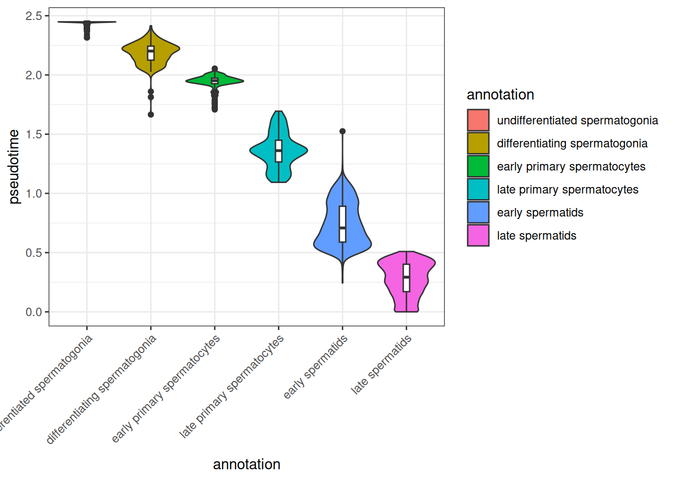
> Check the distribution of pseudotime values across the different cell clusters.
>
> What do you observe? Where you expecting this?
>
> > **NOTE:**
> >
> > ``` r
> > tibble(
> > annotation = germcells$annotation,
> > pseudotime = germcells$pseudotime
> > ) |>
> > ggplot(aes(x = annotation, y = pseudotime, fill = annotation)) +
> > geom_violin(scale = 'width') +
> > geom_boxplot(outlier.shape = NULL, width = 0.1, fill = 'white') +
> > theme_bw() +
> > theme(axis.text.x = element_text(angle = 45, hjust = 1, vjust = 1))
> > ```
> >
> > 
>
> `slingshot` does not know in which direction cells differentiate: the pseudotime may well increase from late spermatids to spermatogonia! Correct pseudotime values, so that they increase along the differentiation. Note that the `start.clus` argument of `slingshot()` can also be used to specify the starting point of a trajectory.
>
> ``` r
> pt <- slingshot::slingPseudotime(germcells_slingshot)[, 'Lineage1']
> first_type <- levels(germcells$annotation)[1]
> last_type <- rev(levels(germcells$annotation))[1]
> if (median(pt[germcells$annotation == first_type], na.rm = TRUE) > median(pt[germcells$annotation == last_type], na.rm = TRUE)) {
> pt <- -1 * pt
> }
> germcells$pseudotime <- scales::rescale(pt, c(0, 1))
> ```
### 15.2.3 BONUS: Daunting snippet but that makes a cool figure for a paper: modeling pseudotime-dependent gene expression
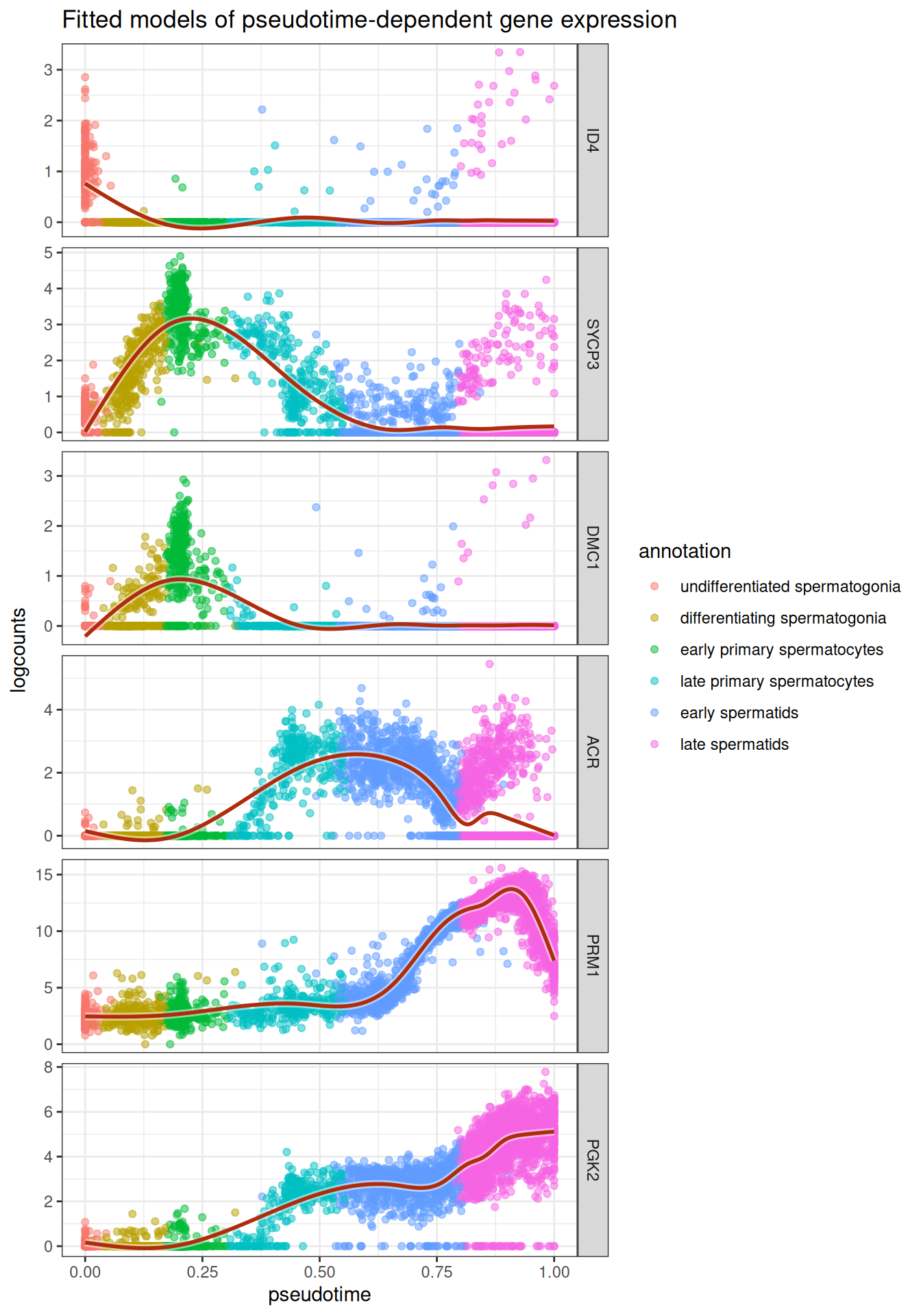
Using pseudotime / cell, one can model gene expression along the differentiation process. This alleviates the need to study gene expression **per cell**, and allows one to focus on process-related effects (e.g. gene expression during a developmental trajectory).
> **NOTE:**
>
> Try to do so for few markers of spermatogonia, spermatocytes and spermatids.
>
> > **NOTE:**
> >
> > ``` r
> > genes <- c('ID4', 'SYCP3', 'DMC1', 'ACR', 'PRM1', 'PGK2')
> > fitExprs <- logcounts(germcells[genes, ]) |> # ----------------------------------- Get norm. counts for genes of interest
> > as.matrix() |>
> > t() |>
> > as_tibble() |>
> > mutate( # ----------------------------------------------------------------- Add information for each cell
> > cellID = colnames(germcells),
> > annotation = germcells$annotation,
> > pseudotime = germcells$pseudotime
> > ) |>
> > filter(!is.na(pseudotime)) |>
> > pivot_longer(all_of(genes), names_to = 'gene', values_to = 'obs_expr') |> # - Pivot in "long" tidy format
> > mutate(gene = factor(gene, genes)) |>
> > group_by(gene) |> # ------------------------------------------------------- Group rows by genes
> > nest() |> # --------------------------------------------------------------- For each gene, extract the subtable into a column named data
> > mutate(
> > gamModel = map(data, ~mgcv::gam(obs_expr ~ s(pseudotime, bs = "cs"), data = .)),
> > gamFitted_expr = map(gamModel, predict) # ------------------------------ For each gene, fit the expression values ~ pseudotime with a GAM
> > ) |>
> > dplyr::select(-ends_with('Model')) |>
> > unnest(c(data, ends_with('_expr'))) # -------------------------------------- Unnest all the modelled expressions
> > ggplot(fitExprs) +
> > geom_point(aes(x = pseudotime, y = obs_expr, col = annotation), alpha = 0.5) +
> > geom_line(aes(x = pseudotime, y = gamFitted_expr), col = 'white', linewidth = 2, alpha = 0.5) +
> > geom_line(aes(x = pseudotime, y = gamFitted_expr), col = '#af2d0c', linewidth = 1) +
> > theme_bw() +
> > facet_grid(gene~., scales = 'free') +
> > labs(y = 'logcounts') +
> > ggtitle('Fitted models of pseudotime-dependent gene expression')
> > ```
> >
> > 
## 15.3 Ordering trajectory with RNA velocity
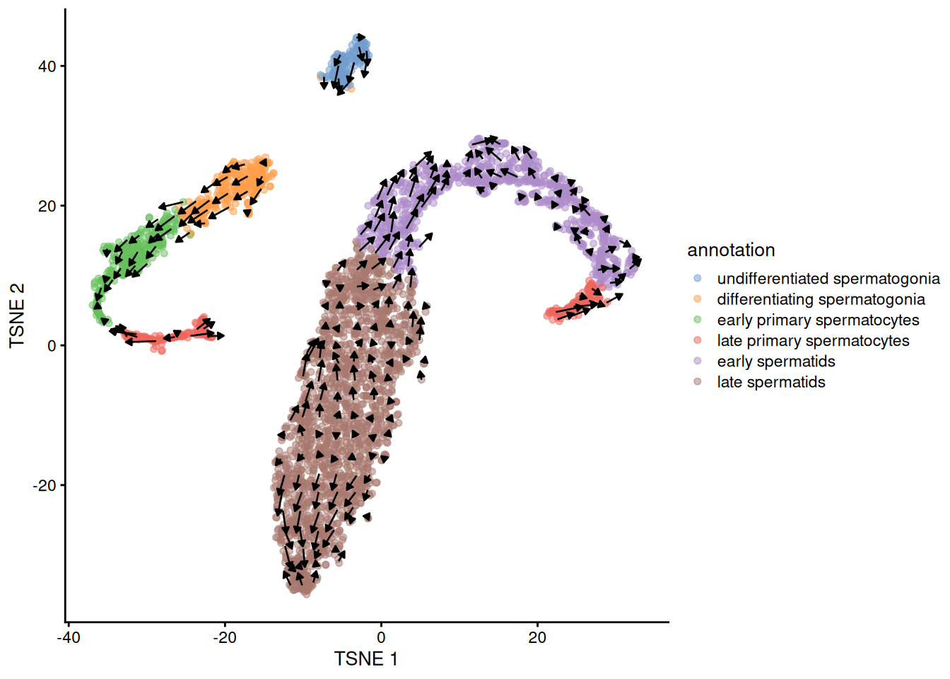
As we saw earlier, TI does not necessarily know which direction is right for a given trajectory. This orientation can be sometimes refined using RNA velocity. Let’s see whether RNA velocity helps orientating our spermatocyte differentiation lineage trajectory here.
> **WARNING:**
>
> RNA velocity requires the counts of spliced and unspliced reads, for each gene in each cell. These counts are not provided in GEO: they were computed from the raw reads of the study with [`velocyto`](https://velocyto.org/). The resulting `loom` file (`Guo_testis_full-counts.loom`, 38 MB) is shipped with this book, and installed in your workshop session: its path is given by `system.file("extdata", "Guo_testis_full-counts.loom", package = "scRNAseqPhysalia2026")`.
>
> `velociraptor` runs [`scVelo`](https://scvelo.readthedocs.io/) (a `python` package) in a dedicated `python` environment, managed by the `basilisk` package: this environment is already installed in your workshop session.
> **NOTE:**
>
> - Read `velociraptor` documentation. What do you need to compute RNA velocity scores in R?
> - Import `spliced` and `unspliced` counts computed with `velocyto` in R.
> - Try and compute RNA velocity.
>
> > **NOTE:**
> >
> > ``` r
> > ## - Import entire GSE112013 dataset with spliced/unspliced counts
> > loom_file <- system.file("extdata", "Guo_testis_full-counts.loom", package = "scRNAseqPhysalia2026")
> > full_GSE112013_counts <- LoomExperiment::import(loom_file)
> > full_GSE112013_counts
> > ## class: LoomExperiment
> > ## dim: 16006 6131
> > ## metadata(8): CreatedWith CreationDate ... velocyto.__version__
> > ## velocyto.logic
> > ## assays(2): spliced unspliced
> > ## rownames: NULL
> > ## rowData names(6): Accession Chromosome ... Start Strand
> > ## colnames(6131): AAACCTGGTGCCTTGG AAACCTGTCAACGGGA ...
> > ## TTTGTCAGTGTGCGTC TTTGTCATCCAAACTG
> > ## colData names(5): Barcode CellID ids ncells sample
> > ## rowGraphs(0): NULL
> > ## colGraphs(0): NULL
> >
> > ## - Filter `germcells` genes and cells to only retain those present in `full_GSE112013_counts`
> > germcells <- germcells[
> > rowData(germcells)$gene_id %in% rowData(full_GSE112013_counts)$Accession,
> > germcells$Barcode %in% full_GSE112013_counts$Barcode
> > ]
> >
> > ## - Reorder rows of `full_GSE112013_counts_germcells` to match those of `germcells`
> > full_GSE112013_counts_germcells <- full_GSE112013_counts[match(rowData(germcells)$gene_id, rowData(full_GSE112013_counts)$Accession), match(germcells$Barcode, full_GSE112013_counts$Barcode)]
> > dim(germcells)
> > ## [1] 15543 3967
> > dim(full_GSE112013_counts_germcells)
> > ## [1] 15543 3967
> >
> > ## - Add spliced/unspliced counts to germcells
> > assay(germcells, 'spliced', withDimnames=FALSE) <- as(assay(full_GSE112013_counts_germcells, 'spliced'), 'dgCMatrix')
> > assay(germcells, 'unspliced', withDimnames=FALSE) <- as(assay(full_GSE112013_counts_germcells, 'unspliced'), 'dgCMatrix')
> > germcells
> > ## class: SingleCellExperiment
> > ## dim: 15543 3967
> > ## metadata(2): scDblFinder.threshold qc
> > ## assays(4): counts logcounts spliced unspliced
> > ## rownames(15543): SAMD11 NOC2L ... DRP2 TRIM49
> > ## rowData names(8): gene_name gene_id ... hvg isHVG
> > ## colnames(3967): Donor2-AAACCTGGTGCCTTGG-1 Donor2-AAACCTGTCAACGGGA-1
> > ## ... Donor1-TTTGTCAGTAAGGGAA-2 Donor1-TTTGTCATCCAAACTG-2
> > ## colData names(18): cellid Barcode ... annotation pseudotime
> > ## reducedDimNames(3): corrected TSNE corrected_2
> > ## mainExpName: NULL
> > ## altExpNames(0):
> >
> > ## - Run velociraptor
> > velo_out <- velociraptor::scvelo(
> > germcells,
> > assay.X = "counts",
> > subset.row = rowData(germcells)$isHVG,
> > use.dimred = "corrected"
> > )
> > ## Registered S3 method overwritten by 'zellkonverter':
> > ## method from
> > ## py_to_r.pandas.core.arrays.categorical.Categorical reticulate
> > ## Using Python: /opt/R-cache/R/BiocBook/envs/scRNAseqPhysalia2026-1d65e4bd55da/bin/python
> > ## Creating virtual environment '/opt/R-cache/R/basilisk/1.25.0/velociraptor/1.23.0/env' ...
> > ## + /opt/R-cache/R/BiocBook/envs/scRNAseqPhysalia2026-1d65e4bd55da/bin/python -m venv /opt/R-cache/R/basilisk/1.25.0/velociraptor/1.23.0/env
> > ## Done!
> > ## Installing packages: pip, wheel, setuptools
> > ## + /opt/R-cache/R/basilisk/1.25.0/velociraptor/1.23.0/env/bin/python -m pip install --upgrade pip wheel setuptools
> > ## Installing packages: 'anndata==0.11.4', 'array-api-compat==1.12.0', 'click==8.2.1', 'contourpy==1.3.2', 'cycler==0.12.1', 'fonttools==4.58.5', 'h5py==3.14.0', 'joblib==1.5.1', 'kiwisolver==1.4.8', 'legacy-api-wrap==1.4.1', 'llvmlite==0.44.0', 'loompy==3.0.8', 'matplotlib==3.10.3', 'natsort==8.4.0', 'networkx==3.5', 'numba==0.61.2', 'numpy==2.2.6', 'numpy-groupies==0.11.3', 'packaging==25.0', 'pandas==2.3.1', 'patsy==1.0.1', 'pillow==11.3.0', 'pip==25.1.1', 'pynndescent==0.5.13', 'pyparsing==3.2.3', 'python-dateutil==2.9.0.post0', 'pytz==2025.2', 'scanpy==1.11.3', 'scikit-learn==1.7.0', 'scipy==1.15.3', 'scvelo==0.3.3', 'seaborn==0.13.2', 'session-info2==0.1.2', 'setuptools==80.9.0', 'six==1.17.0', 'statsmodels==0.14.5', 'threadpoolctl==3.6.0', 'tqdm==4.67.1', 'typing_extensions==4.14.1', 'tzdata==2025.2', 'umap-learn==0.5.9.post2', 'wheel==0.45.1'
> > ## + /opt/R-cache/R/basilisk/1.25.0/velociraptor/1.23.0/env/bin/python -m pip install --upgrade --no-user 'anndata==0.11.4' 'array-api-compat==1.12.0' 'click==8.2.1' 'contourpy==1.3.2' 'cycler==0.12.1' 'fonttools==4.58.5' 'h5py==3.14.0' 'joblib==1.5.1' 'kiwisolver==1.4.8' 'legacy-api-wrap==1.4.1' 'llvmlite==0.44.0' 'loompy==3.0.8' 'matplotlib==3.10.3' 'natsort==8.4.0' 'networkx==3.5' 'numba==0.61.2' 'numpy==2.2.6' 'numpy-groupies==0.11.3' 'packaging==25.0' 'pandas==2.3.1' 'patsy==1.0.1' 'pillow==11.3.0' 'pip==25.1.1' 'pynndescent==0.5.13' 'pyparsing==3.2.3' 'python-dateutil==2.9.0.post0' 'pytz==2025.2' 'scanpy==1.11.3' 'scikit-learn==1.7.0' 'scipy==1.15.3' 'scvelo==0.3.3' 'seaborn==0.13.2' 'session-info2==0.1.2' 'setuptools==80.9.0' 'six==1.17.0' 'statsmodels==0.14.5' 'threadpoolctl==3.6.0' 'tqdm==4.67.1' 'typing_extensions==4.14.1' 'tzdata==2025.2' 'umap-learn==0.5.9.post2' 'wheel==0.45.1'
> > ## Virtual environment '/opt/R-cache/R/basilisk/1.25.0/velociraptor/1.23.0/env' successfully created.
> > ## computing moments based on connectivities
> > ## finished (0:00:00) --> added
> > ## 'Ms' and 'Mu', moments of un/spliced abundances (adata.layers)
> > ## computing velocities
> > ## finished (0:00:00) --> added
> > ## 'velocity', velocity vectors for each individual cell (adata.layers)
> > ## computing velocity graph (using 1/4 cores)
> > ## WARNING: Unable to create progress bar. Consider installing `tqdm` as `pip install tqdm` and `ipywidgets` as `pip install ipywidgets`,
> > ## or disable the progress bar using `show_progress_bar=False`.
> > ## finished (0:00:02) --> added
> > ## 'velocity_graph', sparse matrix with cosine correlations (adata.uns)
> > ## computing terminal states
> > ## identified 6 regions of root cells and 3 regions of end points .
> > ## finished (0:00:00) --> added
> > ## 'root_cells', root cells of Markov diffusion process (adata.obs)
> > ## 'end_points', end points of Markov diffusion process (adata.obs)
> > ## --> added 'velocity_length' (adata.obs)
> > ## --> added 'velocity_confidence' (adata.obs)
> > ## --> added 'velocity_confidence_transition' (adata.obs)
> > ## For native R and reading and writing of H5AD files, an R object,
> > ## and conversion to or objects, check out the
> > ## anndataR package:
> > ## ℹ Install it from Bioconductor with `BiocManager::install("anndataR")`
> > ## ℹ See more at
> > ## This message is displayed once per session.
> > velo_out
> > ## class: SingleCellExperiment
> > ## dim: 1955 3967
> > ## metadata(4): neighbors velocity_params velocity_graph
> > ## velocity_graph_neg
> > ## assays(6): X spliced ... Mu velocity
> > ## rownames(1955): C1orf159 TTLL10 ... COL6A2 SPATC1L
> > ## rowData names(4): velocity_gamma velocity_qreg_ratio velocity_r2
> > ## velocity_genes
> > ## colnames(3967): Donor2-AAACCTGGTGCCTTGG-1 Donor2-AAACCTGTCAACGGGA-1
> > ## ... Donor1-TTTGTCAGTAAGGGAA-2 Donor1-TTTGTCATCCAAACTG-2
> > ## colData names(7): velocity_self_transition root_cells ...
> > ## velocity_confidence velocity_confidence_transition
> > ## reducedDimNames(1): X_pca
> > ## mainExpName: NULL
> > ## altExpNames(0):
> > ```
- **Embed the velocity field in tSNE scRNAseq embedding and plot the RNA velocity field on top of tSNE projection. Conclude.**
``` r
embedded_velo <- velociraptor::embedVelocity(reducedDim(germcells, "TSNE"), velo_out)
## ℹ Using the 'X' assay as the X matrix
## computing velocity embedding
## finished (0:00:00) --> added
## 'velocity_target', embedded velocity vectors (adata.obsm)
head(embedded_velo)
## [,1] [,2]
## [1,] -0.004190276 0.62071260
## [2,] -0.182686754 -0.42189365
## [3,] -0.092559296 0.13643846
## [4,] -0.344845658 -0.38175330
## [5,] -0.056569775 -0.03182575
## [6,] 0.279834642 0.37126586
grid_df <- velociraptor::gridVectors(reducedDim(germcells, "TSNE"), embedded_velo, resolution = 30, scale = TRUE)
head(grid_df)
## start.TSNE1 start.TSNE2 end.TSNE1 end.TSNE2
## 1 17.6814096 26.505914 16.7363358 28.448114
## 2 -10.5292413 -18.545300 -10.9718974 -20.662721
## 3 -3.2539728 -13.097256 -3.6592306 -12.211134
## 4 -7.9481561 -18.364766 -8.6062669 -20.702600
## 5 -0.7843155 2.813711 -0.7006013 3.094165
## 6 -5.6143385 10.685881 -4.5985983 12.160603
scater::plotReducedDim(germcells, 'TSNE', colour_by = "annotation", point_alpha = 0.5) +
geom_segment(
data = grid_df,
mapping = aes(x = start.TSNE1, y = start.TSNE2, xend = end.TSNE1, yend = end.TSNE2),
arrow = arrow(length = unit(0.05, "inches"), type = "closed")
)
```
## 15.4 Session info
> **NOTE:**
>
> ## ─ Session info ────────────────────────────────────────────────────────────
> ## setting value
> ## version R version 4.6.1 (2026-06-24)
> ## os Ubuntu 24.04.5 LTS
> ## system x86_64, linux-gnu
> ## ui X11
> ## language (EN)
> ## collate C
> ## ctype en_US.UTF-8
> ## tz Etc/UTC
> ## date 2026-11-13
> ## pandoc 3.13 @ /usr/bin/ (via rmarkdown)
> ## quarto 1.11.5 @ /usr/local/bin/quarto
> ##
> ## ─ Packages ────────────────────────────────────────────────────────────────
> ## package * version date (UTC) lib source
> ## abind 1.4-8 2024-09-12 [2] RSPM (R 4.6.0)
> ## AnnotationDbi 1.75.2 2026-07-21 [2] Bioconductor 3.24 (R 4.6.1)
> ## basilisk 1.25.0 2026-04-29 [2] Bioconductor 3.24 (R 4.6.1)
> ## batchelor 1.29.0 2026-04-28 [2] Bioconductor 3.24 (R 4.6.1)
> ## beachmat 2.29.3 2026-09-23 [2] Bioconductor 3.24 (R 4.6.1)
> ## beeswarm 0.4.0 2021-06-01 [2] RSPM (R 4.6.0)
> ## Biobase * 2.73.2 2026-07-29 [2] Bioconductor 3.24 (R 4.6.1)
> ## BiocBaseUtils 1.15.1 2026-05-10 [2] Bioconductor 3.24 (R 4.6.1)
> ## BiocFileCache * 3.3.3 2026-11-11 [2] Bioconductor 3.24 (R 4.6.1)
> ## BiocGenerics * 0.59.13 2026-11-11 [2] Bioconductor 3.24 (R 4.6.1)
> ## BiocIO 1.23.3 2026-04-29 [2] Bioconductor 3.24 (R 4.6.1)
> ## BiocNeighbors 2.7.3 2026-08-21 [2] Bioconductor 3.24 (R 4.6.1)
> ## BiocParallel 1.47.0 2026-04-28 [2] Bioconductor 3.24 (R 4.6.1)
> ## BiocSingular 1.29.2 2026-10-08 [2] Bioconductor 3.24 (R 4.6.1)
> ## Biostrings 2.81.9 2026-09-06 [2] Bioconductor 3.24 (R 4.6.1)
> ## bit 4.6.0 2025-03-06 [2] RSPM (R 4.6.0)
> ## bit64 4.8.6 2026-09-01 [2] RSPM (R 4.6.0)
> ## bitops 1.1-0 2026-07-30 [2] RSPM (R 4.6.0)
> ## blob 1.3.0 2026-01-14 [2] RSPM (R 4.6.0)
> ## bluster 1.23.1 2026-08-25 [2] Bioconductor 3.24 (R 4.6.1)
> ## cachem 1.1.0 2024-05-16 [2] RSPM (R 4.6.0)
> ## cigarillo 1.3.1 2026-07-13 [2] Bioconductor 3.24 (R 4.6.1)
> ## cli 3.6.6 2026-04-09 [2] RSPM (R 4.6.0)
> ## cluster 2.1.8.3 2026-07-30 [2] RSPM (R 4.6.1)
> ## codetools 0.2-20 2024-03-31 [3] CRAN (R 4.6.1)
> ## cowplot 1.2.0 2025-07-07 [2] RSPM (R 4.6.0)
> ## crayon 1.5.3 2024-06-20 [2] RSPM (R 4.6.0)
> ## curl 8.1.0 2026-10-14 [2] RSPM (R 4.6.0)
> ## data.table 1.18.6.1 2026-08-24 [2] RSPM (R 4.6.0)
> ## DBI 1.3.0 2026-02-25 [2] RSPM (R 4.6.0)
> ## dbplyr * 2.6.0 2026-06-17 [2] RSPM (R 4.6.0)
> ## DelayedArray 0.39.8 2026-09-30 [2] Bioconductor 3.24 (R 4.6.1)
> ## DelayedMatrixStats 1.35.0 2026-04-28 [2] Bioconductor 3.24 (R 4.6.1)
> ## dichromat 2.0-1 2026-07-22 [2] RSPM (R 4.6.0)
> ## digest 0.6.39 2025-11-19 [2] RSPM (R 4.6.0)
> ## dir.expiry 1.21.0 2026-04-28 [2] Bioconductor 3.24 (R 4.6.1)
> ## dplyr * 1.2.1 2026-04-03 [2] RSPM (R 4.6.0)
> ## dqrng 0.4.1 2024-05-28 [2] RSPM (R 4.6.0)
> ## edgeR 4.99.12 2026-11-04 [2] Bioconductor 3.24 (R 4.6.1)
> ## evaluate 1.0.5 2025-08-27 [2] RSPM (R 4.6.0)
> ## farver 2.1.2 2024-05-13 [2] RSPM (R 4.6.0)
> ## fastmap 1.2.0 2024-05-15 [2] RSPM (R 4.6.0)
> ## filelock 1.0.3 2023-12-11 [2] RSPM (R 4.6.0)
> ## forcats * 1.0.1 2025-09-25 [2] RSPM (R 4.6.0)
> ## generics * 0.1.4 2025-05-09 [2] RSPM (R 4.6.0)
> ## GenomeInfoDb 1.49.1 2026-05-24 [2] Bioconductor 3.24 (R 4.6.1)
> ## GenomicAlignments 1.49.2 2026-09-02 [2] Bioconductor 3.24 (R 4.6.1)
> ## GenomicRanges * 1.65.4 2026-09-02 [2] Bioconductor 3.24 (R 4.6.1)
> ## ggbeeswarm 0.7.3 2025-11-29 [2] RSPM (R 4.6.0)
> ## ggplot2 * 4.0.3 2026-04-22 [2] RSPM (R 4.6.0)
> ## ggrepel 0.9.8 2026-03-17 [2] RSPM (R 4.6.0)
> ## glue 1.8.1 2026-04-17 [2] RSPM (R 4.6.0)
> ## gridExtra 2.3.1 2026-06-25 [2] RSPM (R 4.6.0)
> ## gtable 0.3.6 2024-10-25 [2] RSPM (R 4.6.0)
> ## h5mread 1.5.3 2026-09-02 [2] Bioconductor 3.24 (R 4.6.1)
> ## HDF5Array 1.41.3 2026-08-21 [2] Bioconductor 3.24 (R 4.6.1)
> ## hms 1.1.4 2025-10-17 [2] RSPM (R 4.6.0)
> ## htmltools 0.5.9 2025-12-04 [2] RSPM (R 4.6.0)
> ## htmlwidgets 1.6.4 2023-12-06 [2] RSPM (R 4.6.0)
> ## httr 1.4.9 2026-09-01 [2] RSPM (R 4.6.0)
> ## httr2 1.3.0 2026-07-13 [2] RSPM (R 4.6.0)
> ## igraph 2.3.4 2026-09-30 [2] RSPM (R 4.6.0)
> ## IRanges * 2.47.5 2026-08-27 [2] Bioconductor 3.24 (R 4.6.1)
> ## irlba 2.4.1 2026-10-05 [2] RSPM (R 4.6.0)
> ## jsonlite 2.0.0 2025-03-27 [2] RSPM (R 4.6.0)
> ## KEGGREST 1.53.6 2026-07-23 [2] Bioconductor 3.24 (R 4.6.1)
> ## knitr 1.52 2026-09-06 [2] RSPM (R 4.6.0)
> ## labeling 0.4.3 2023-08-29 [2] RSPM (R 4.6.0)
> ## lattice 0.23-1 2026-08-12 [2] RSPM (R 4.6.1)
> ## lifecycle 1.0.5 2026-01-08 [2] RSPM (R 4.6.0)
> ## limma 3.99.4 2026-11-04 [2] Bioconductor 3.24 (R 4.6.1)
> ## LoomExperiment 1.31.0 2026-04-29 [2] Bioconductor 3.24 (R 4.6.1)
> ## lubridate * 1.9.5 2026-02-04 [2] RSPM (R 4.6.0)
> ## magrittr 2.0.5 2026-04-04 [2] RSPM (R 4.6.0)
> ## MASS 7.3-66 2026-07-15 [2] RSPM (R 4.6.1)
> ## Matrix 1.7-6 2026-07-25 [2] RSPM (R 4.6.1)
> ## MatrixGenerics * 1.25.0 2026-04-28 [2] Bioconductor 3.24 (R 4.6.1)
> ## matrixStats * 1.5.0 2025-01-07 [2] RSPM (R 4.6.0)
> ## memoise 2.0.1 2021-11-26 [2] RSPM (R 4.6.0)
> ## metapod 1.21.0 2026-04-28 [2] Bioconductor 3.24 (R 4.6.1)
> ## mgcv 1.9-4 2025-11-07 [3] CRAN (R 4.6.1)
> ## nlme 3.1-171 2026-09-01 [2] RSPM (R 4.6.1)
> ## org.Hs.eg.db 3.24.6 2026-11-13 [2] Bioconductor
> ## otel 0.2.0 2025-08-29 [2] RSPM (R 4.6.0)
> ## pillar 1.11.1 2025-09-17 [2] RSPM (R 4.6.0)
> ## pkgconfig 2.0.3 2019-09-22 [2] RSPM (R 4.6.0)
> ## png 0.1-9 2026-03-15 [2] RSPM (R 4.6.0)
> ## princurve 2.1.6 2021-01-18 [2] RSPM (R 4.6.0)
> ## purrr * 1.2.2 2026-04-10 [2] RSPM (R 4.6.0)
> ## R.methodsS3 1.8.2 2022-06-13 [2] RSPM (R 4.6.0)
> ## R.oo 1.27.1 2025-05-02 [2] RSPM (R 4.6.0)
> ## R.utils 2.13.0 2025-02-24 [2] RSPM (R 4.6.0)
> ## R6 2.6.1 2025-02-15 [2] RSPM (R 4.6.0)
> ## RColorBrewer 1.1-3 2022-04-03 [2] RSPM (R 4.6.0)
> ## Rcpp 1.1.2 2026-07-05 [2] RSPM (R 4.6.0)
> ## RCurl 1.98-1.20 2026-08-21 [2] RSPM (R 4.6.0)
> ## readr * 2.2.0 2026-02-19 [2] RSPM (R 4.6.0)
> ## ResidualMatrix 1.23.0 2026-04-28 [2] Bioconductor 3.24 (R 4.6.1)
> ## restfulr 0.0.17 2026-06-11 [2] RSPM (R 4.6.0)
> ## reticulate 1.47.0 2026-09-03 [2] RSPM (R 4.6.0)
> ## rhdf5 2.57.20 2026-10-06 [2] Bioconductor 3.24 (R 4.6.1)
> ## rhdf5filters 1.25.5 2026-10-28 [2] Bioconductor 3.24 (R 4.6.1)
> ## Rhdf5lib 2.1.0 2026-04-28 [2] Bioconductor 3.24 (R 4.6.1)
> ## rjson 0.2.23 2024-09-16 [2] RSPM (R 4.6.0)
> ## rlang 1.3.0 2026-07-05 [2] RSPM (R 4.6.0)
> ## rmarkdown 2.32 2026-09-01 [2] RSPM (R 4.6.0)
> ## Rsamtools 2.29.0 2026-04-28 [2] Bioconductor 3.24 (R 4.6.1)
> ## RSQLite 3.53.3 2026-06-30 [2] RSPM (R 4.6.0)
> ## rsvd 1.0.6 2026-10-17 [2] RSPM (R 4.6.0)
> ## rtracklayer 1.73.0 2026-04-28 [2] Bioconductor 3.24 (R 4.6.1)
> ## Rtsne 0.17 2023-12-07 [2] RSPM (R 4.6.0)
> ## S4Arrays 1.13.2 2026-09-30 [2] Bioconductor 3.24 (R 4.6.1)
> ## S4Vectors * 0.51.10 2026-09-16 [2] Bioconductor 3.24 (R 4.6.1)
> ## S7 0.2.2 2026-04-22 [2] RSPM (R 4.6.0)
> ## ScaledMatrix 1.21.0 2026-04-28 [2] Bioconductor 3.24 (R 4.6.1)
> ## scales 1.4.0 2025-04-24 [2] RSPM (R 4.6.0)
> ## scater 1.41.3 2026-10-25 [2] Bioconductor 3.24 (R 4.6.1)
> ## scDblFinder 1.27.12 2026-10-14 [2] Bioconductor 3.24 (R 4.6.1)
> ## scran 1.41.1 2026-05-20 [2] Bioconductor 3.24 (R 4.6.1)
> ## scrapper 1.7.11 2026-11-04 [2] Bioconductor 3.24 (R 4.6.1)
> ## scuttle 1.23.2 2026-08-27 [2] Bioconductor 3.24 (R 4.6.1)
> ## Seqinfo * 1.3.2 2026-08-27 [2] Bioconductor 3.24 (R 4.6.1)
> ## sessioninfo 1.2.4 2026-06-04 [2] RSPM (R 4.6.0)
> ## SingleCellExperiment * 1.35.2 2026-07-16 [2] Bioconductor 3.24 (R 4.6.1)
> ## SingleR 2.15.4 2026-09-10 [2] Bioconductor 3.24 (R 4.6.1)
> ## slingshot 2.21.0 2026-04-28 [2] Bioconductor 3.24 (R 4.6.1)
> ## SparseArray 1.13.4 2026-09-30 [2] Bioconductor 3.24 (R 4.6.1)
> ## sparseMatrixStats 1.25.0 2026-04-28 [2] Bioconductor 3.24 (R 4.6.1)
> ## statmod 1.5.2 2026-05-17 [2] RSPM (R 4.6.0)
> ## stringi 1.8.9 2026-08-04 [2] RSPM (R 4.6.0)
> ## stringr * 1.6.0 2025-11-04 [2] RSPM (R 4.6.0)
> ## SummarizedExperiment * 1.43.0 2026-04-28 [2] Bioconductor 3.24 (R 4.6.1)
> ## tibble * 3.3.1 2026-01-11 [2] RSPM (R 4.6.0)
> ## tidyr * 1.3.2 2025-12-19 [2] RSPM (R 4.6.0)
> ## tidyselect 1.2.1 2024-03-11 [2] RSPM (R 4.6.0)
> ## tidyverse * 2.0.0 2023-02-22 [2] RSPM (R 4.6.0)
> ## timechange 0.4.0 2026-01-29 [2] RSPM (R 4.6.0)
> ## TrajectoryUtils 1.21.0 2026-04-28 [2] Bioconductor 3.24 (R 4.6.1)
> ## tzdb 0.5.0 2025-03-15 [2] RSPM (R 4.6.0)
> ## UCSC.utils 1.9.0 2026-04-28 [2] Bioconductor 3.24 (R 4.6.1)
> ## vctrs 0.7.3 2026-04-11 [2] RSPM (R 4.6.0)
> ## velociraptor 1.23.0 2026-04-29 [2] Bioconductor 3.24 (R 4.6.1)
> ## vipor 0.4.7 2023-12-18 [2] RSPM (R 4.6.0)
> ## viridis 0.6.5 2024-01-29 [2] RSPM (R 4.6.0)
> ## viridisLite 0.4.3 2026-02-04 [2] RSPM (R 4.6.0)
> ## vroom 1.7.1 2026-03-31 [2] RSPM (R 4.6.0)
> ## withr 3.0.3 2026-06-19 [2] RSPM (R 4.6.0)
> ## xfun 0.62 2026-10-16 [2] RSPM (R 4.6.0)
> ## xgboost 3.2.1.1 2026-03-18 [2] RSPM (R 4.6.0)
> ## XML 3.99-0.25 2026-09-27 [2] RSPM (R 4.6.0)
> ## XVector 0.53.0 2026-04-28 [2] Bioconductor 3.24 (R 4.6.1)
> ## yaml 2.3.12 2025-12-10 [2] RSPM (R 4.6.0)
> ## zellkonverter 1.23.1 2026-11-10 [2] Bioconductor 3.24 (R 4.6.1)
> ##
> ## [1] /tmp/RtmpyQdi1U/Rinstc2e9543f3
> ## [2] /usr/local/lib/R/site-library
> ## [3] /usr/local/lib/R/library
> ## * ── Packages attached to the search path.
> ##
> ## ─ Python configuration ────────────────────────────────────────────────────
> ## python: /opt/R-cache/R/basilisk/1.25.0/velociraptor/1.23.0/env/bin/python
> ## libpython: /opt/R-cache/R/BiocBook/envs/scRNAseqPhysalia2026-1d65e4bd55da/lib/libpython3.12.so
> ## pythonhome: /opt/R-cache/R/basilisk/1.25.0/velociraptor/1.23.0/env:/opt/R-cache/R/basilisk/1.25.0/velociraptor/1.23.0/env
> ## version: 3.12.16 (main, Oct 26 2026, 11:37:43) [GCC 15.3.0]
> ## numpy: /opt/R-cache/R/basilisk/1.25.0/velociraptor/1.23.0/env/lib/python3.12/site-packages/numpy
> ## numpy_version: 2.2.6
> ##
> ## NOTE: Python version was forced by use_python() function
> ##
> ## ───────────────────────────────────────────────────────────────────────────