Text mining and sentiment analysis in R
Pre-processing LOTR text in R
Complete LOTR text can be downloaded from Kaggle: https://www.kaggle.com/ashishsinhaiitr/lord-of-the-rings-text. I edited the text very quickly, by simply removing the foreword and name of each of the 3 tomes. I also added the “book” II to VI (there was only an entry for “Book I”, the others were missing). Finally, I collated the three tomes together.
library(tidyverse)## ── Attaching packages ───────────────────────────────────────────────────────────────────────────────────────────────────────────────────────────────────────────────────────────────────────────────────────────────────────────── tidyverse 1.3.0 ──## ✔ ggplot2 3.3.3 ✔ purrr 0.3.4
## ✔ tibble 3.0.5 ✔ dplyr 1.0.3
## ✔ tidyr 1.1.2 ✔ stringr 1.4.0
## ✔ readr 1.4.0 ✔ forcats 0.5.0## ── Conflicts ──────────────────────────────────────────────────────────────────────────────────────────────────────────────────────────────────────────────────────────────────────────────────────────────────────────────── tidyverse_conflicts() ──
## ✖ dplyr::filter() masks stats::filter()
## ✖ dplyr::lag() masks stats::lag()library(magrittr)##
## Attaching package: 'magrittr'## The following object is masked from 'package:purrr':
##
## set_names## The following object is masked from 'package:tidyr':
##
## extract# -- FUNCTIONS ----------------------
fillUpLines <- function(lines) {
res <- lapply(1:sum(lines), function(K) {
value <- which(lines)[K]
n_reps <- ifelse(
K < sum(lines),
which(lines)[K+1] - which(lines)[K],
length(lines) - which(lines)[K] + 1
)
res <- rep(value, n_reps)
return(res)
})
res <- do.call(c, res)
res <- c(rep(NA, length(lines) - length(res)), res)
return(res)
}
parseBook <- function(txt_path) {
txt <- readLines(txt_path) %>%
tibble(
line = 1:length(.),
text = .
) %>%
filter(text != "") %>%
mutate(line = 1:nrow(.))
line_tomes <- txt$text %>% str_detect("0. - The ")
line_books <- txt$text %>% str_detect("BOOK")
line_chapters <- txt$text %>% str_detect("_Chapter")
line_chapter_titles <- 1:nrow(txt) %in% {which(line_chapters) + 1}
txt %<>%
mutate(text = gsub('_', '', text)) %>%
mutate(tome = fillUpLines(line_tomes) %>% txt$text[.] %>% gsub('^\\s+|_', '', .)) %>%
mutate(book = fillUpLines(line_books) %>% txt$text[.] %>% gsub('^\\s+|_', '', .)) %>%
mutate(chapter = fillUpLines(line_chapters) %>% txt$text[.] %>% gsub('^\\s+|_', '', .)) %>%
mutate(chapter_title = fillUpLines(line_chapter_titles) %>% txt$text[.] %>% gsub('^\\s+|_', '', .)) %>%
mutate(raw_text = text) %>%
mutate(text = gsub('^\\s+', '', raw_text)) %>%
mutate(nchar = nchar(text))
txt$entry <- "corpus"
txt$entry[line_tomes] <- "tome"
txt$entry[line_books] <- "book"
txt$entry[line_chapters] <- "chapter"
txt$entry[line_chapter_titles] <- "chapter_title"
txt[txt$entry != 'corpus', ] %<>% mutate(book = NA, chapter = NA, chapter_title = NA)
return(txt)
}
# // FUNCTIONS ----------------------
txt_path <- 'txt/collated_books.txt'
LOTR <- parseBook(txt_path)Let’s have a look at how the different books are structued. This is a nice little tidyverse-assisted data wrangling exercise. First, let’s see how many characters each chapter contains.
LOTR %>%
    group_by(tome, book, chapter, chapter_title) %>%
    tally(nchar) %>%
    filter(!is.na(chapter) & !is.na(book)) %>%
    ggplot(aes(x = chapter, y = n, fill = chapter)) +
    geom_col() +
    theme_light() +
    facet_wrap(~book, scales = "free") +
    theme(axis.text.x = element_text(angle = 45, hjust = 1, vjust = 1)) +
    labs(x = 'Chapter', y = '# of character / chapter', title = "Number of character per chapter")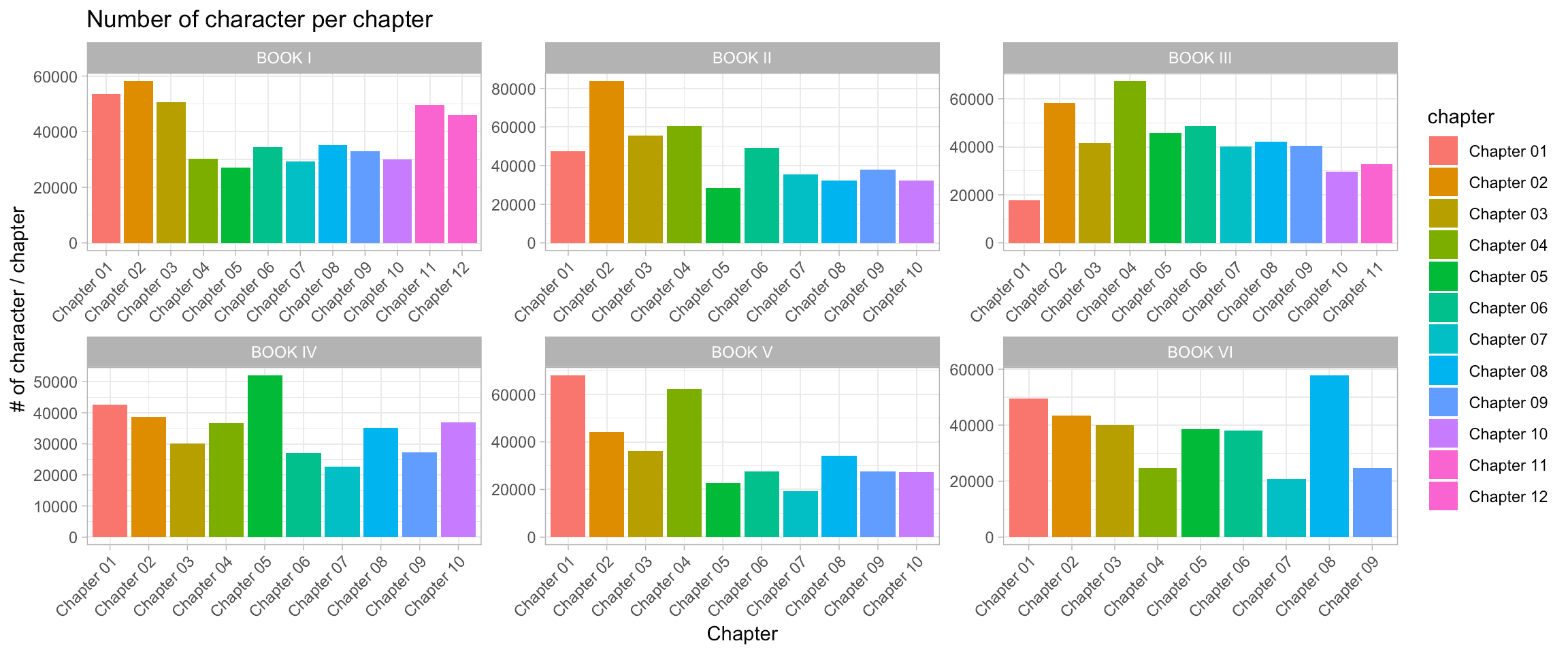
There are some pretty big discrepancies between the length of each chapter in LOTR books. Now, let’s see whether Tolkien was more consistent in the length of paragraphs in each book.
LOTR %>%
    filter(!is.na(chapter) & !is.na(book)) %>%
    ggplot(aes(x = chapter, y = nchar, fill = chapter)) +
    geom_violin() +
    ggbeeswarm::geom_beeswarm(alpha = 0.2, size = 0.4, fill = NA, col = 'black') +
    geom_boxplot(fill = 'white', width = 0.2, outlier.shape = NA) +
    theme_light() +
    facet_wrap(~book, scales = "free") +
    scale_y_log10() +
    annotation_logticks(sides = 'l') +
    theme(axis.text.x = element_text(angle = 45, hjust = 1, vjust = 1)) +
    labs(x = 'Chapter', y = '# of character / paragraph', title = "Number of character per paragraph")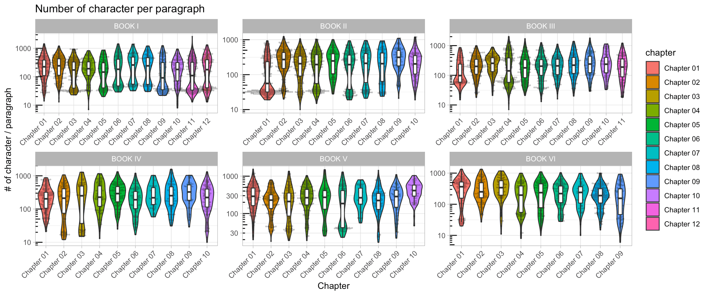
Quite interesting: some chapters (especially in Book I) have a stricking bi-modal distribution. Some “paragraphs” look like they are under 100 character each. If you dig into it, you’ll realize that these paragraphs are actually the songs/poems that are mostly found in the first tome of LOTR, notably when the hobbits encounter Tom Bombabil (one of my favorite chapters in the entire saga!).
Let’s confirm this quickly. After visual inspection of the text file, the songs mostly start with a repetition of 10 to 12 spaces ().
bool <- grepl("^          [a-zA-Z]|^           [a-zA-Z]|^            [a-zA-Z]", LOTR$raw_text)
LOTR[bool & LOTR$entry == "corpus", "entry"] <- "song"
LOTR %>%
    filter(!is.na(chapter) & !is.na(book)) %>%
    ggplot(aes(x = chapter, y = nchar, fill = chapter)) +
    ggbeeswarm::geom_beeswarm(
        alpha = 0.4,
        size = 0.6,
        fill = NA,
        aes(col = entry)
    ) +
    theme_light() +
    facet_wrap(~book, scales = "free") +
    scale_y_log10() +
    annotation_logticks(sides = 'l') +
    theme(axis.text.x = element_text(angle = 45, hjust = 1, vjust = 1)) +
    labs(x = 'Chapter', y = '# of character / paragraph', title = "Number of character per paragraph")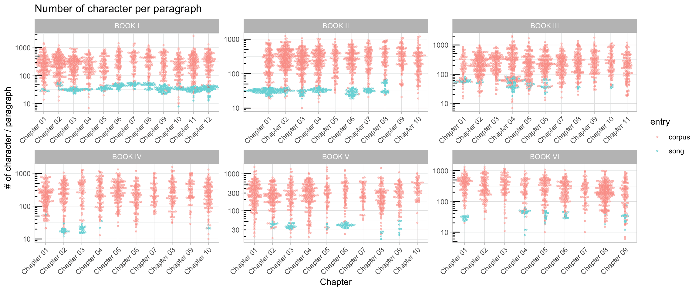
Converting the tibble into an even tidier format with tidytext
The tidytext package is very useful to transform a tibble containing strings into a tidier tibble, with only 1 word per row. This is done with the unnest_tokens() function:
library(tidytext)
LOTR
## # A tibble: 9,162 x 9
## line text tome book chapter chapter_title raw_text nchar entry
## <int> <chr> <chr> <chr> <chr> <chr> <chr> <int> <chr>
## 1 1 01 - The … 01 - T… <NA> <NA> <NA> " … 31 tome
## 2 2 BOOK I 01 - T… <NA> <NA> <NA> " … 6 book
## 3 3 Chapter 01 01 - T… <NA> <NA> <NA> " … 10 chap…
## 4 4 A Long-ex… 01 - T… <NA> <NA> <NA> " … 21 chap…
## 5 5 When Mr. … 01 - T… BOOK… Chapte… A Long-expec… " When … 194 corp…
## 6 6 Bilbo was… 01 - T… BOOK… Chapte… A Long-expec… " Bilbo… 868 corp…
## 7 7 'It will … 01 - T… BOOK… Chapte… A Long-expec… " 'It w… 90 corp…
## 8 8 But so fa… 01 - T… BOOK… Chapte… A Long-expec… " But s… 416 corp…
## 9 9 The eldes… 01 - T… BOOK… Chapte… A Long-expec… " The e… 580 corp…
## 10 10 Twelve mo… 01 - T… BOOK… Chapte… A Long-expec… " Twelv… 451 corp…
## # … with 9,152 more rowsLOTR %>%
unnest_tokens(word, text)## # A tibble: 471,247 x 9
## line tome book chapter chapter_title raw_text nchar entry word
## <int> <chr> <chr> <chr> <chr> <chr> <int> <chr> <chr>
## 1 1 01 - The… <NA> <NA> <NA> " … 31 tome 01
## 2 1 01 - The… <NA> <NA> <NA> " … 31 tome the
## 3 1 01 - The… <NA> <NA> <NA> " … 31 tome fell…
## 4 1 01 - The… <NA> <NA> <NA> " … 31 tome of
## 5 1 01 - The… <NA> <NA> <NA> " … 31 tome the
## 6 1 01 - The… <NA> <NA> <NA> " … 31 tome ring
## 7 2 01 - The… <NA> <NA> <NA> " … 6 book book
## 8 2 01 - The… <NA> <NA> <NA> " … 6 book i
## 9 3 01 - The… <NA> <NA> <NA> " … 10 chap… chap…
## 10 3 01 - The… <NA> <NA> <NA> " … 10 chap… 01
## # … with 471,237 more rowsTo illustrate the use of tidytext and how well it can be used with tidyverse-related tools, we can count how many times each character is named in each chapter:
characters <- c('frodo', 'sam', 'gandalf', 'aragorn', 'pippin', 'merry', 'gimli', 'legolas', 'gollum', 'bilbo')
LOTR %>%
unnest_tokens(word, text) %>%
filter(!is.na(chapter) & !is.na(book)) %>%
filter(word %in% characters) %>%
mutate(word = factor(word, characters)) %>%
count(tome, book, chapter, chapter_title, word) %>%
ggplot(aes(x = chapter, y = n, fill = chapter)) +
geom_col() +
theme_light() +
facet_grid(word~book, scales = "free") +
theme(axis.text.x = element_text(angle = 45, hjust = 1, vjust = 1)) +
labs(x = 'Chapter', y = '# of character citations', title = "Number of times each protagonist is named")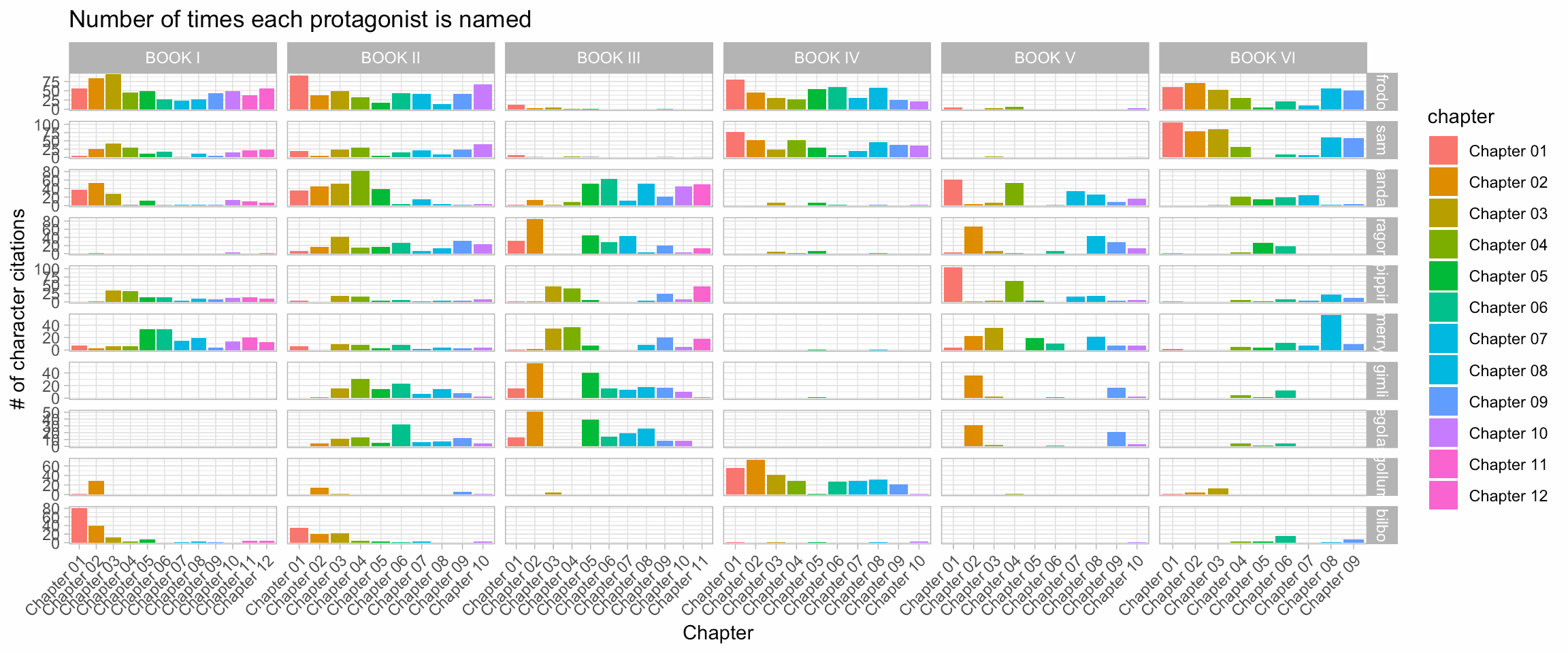
I love this figure. In just a few lines of code, the number of times each protagonist is named, in each chapter of each book, is computed and beautifully plotted. Just looking at this figure, I could tell what happens in each chapter:
- Book III, chapters 2 and 3 are most likely about Merry and Pippins when they are captured by the Orcs;
- In Book V, Chapter 4, Pippin and Gandalf are together, defending Minas Tirith;
- The return of Gollum in the third chapter of Book 6 signs the achievement of the quest with Gollum falling into the Cracks of Doom.
And here is another type of representation of the # of occurence of each protagonist. The input data.frame stays the same, I’ve just changed a tiny bit the ggplot2 geometries, et voila!
characters <- c('frodo', 'sam', 'gandalf', 'aragorn', 'pippin', 'merry', 'gimli', 'legolas', 'gollum', 'bilbo')
LOTR %>%
    unnest_tokens(word, text) %>%
    filter(!is.na(chapter) & !is.na(book)) %>%
    filter(word %in% characters) %>%
    mutate(word = factor(word, characters)) %>%
    count(tome, book, chapter, chapter_title, word) %>%
    ggplot(aes(x = chapter, y = n, fill = word)) +
    geom_col(position = 'fill') +
    facet_grid(~book, scales = "free") +
    theme_light() +
    theme(axis.text.x = element_text(angle = 45, hjust = 1, vjust = 1)) +
    labs(x = 'Chapter', y = '# of character citations', title = "Number of times each protagonist is named")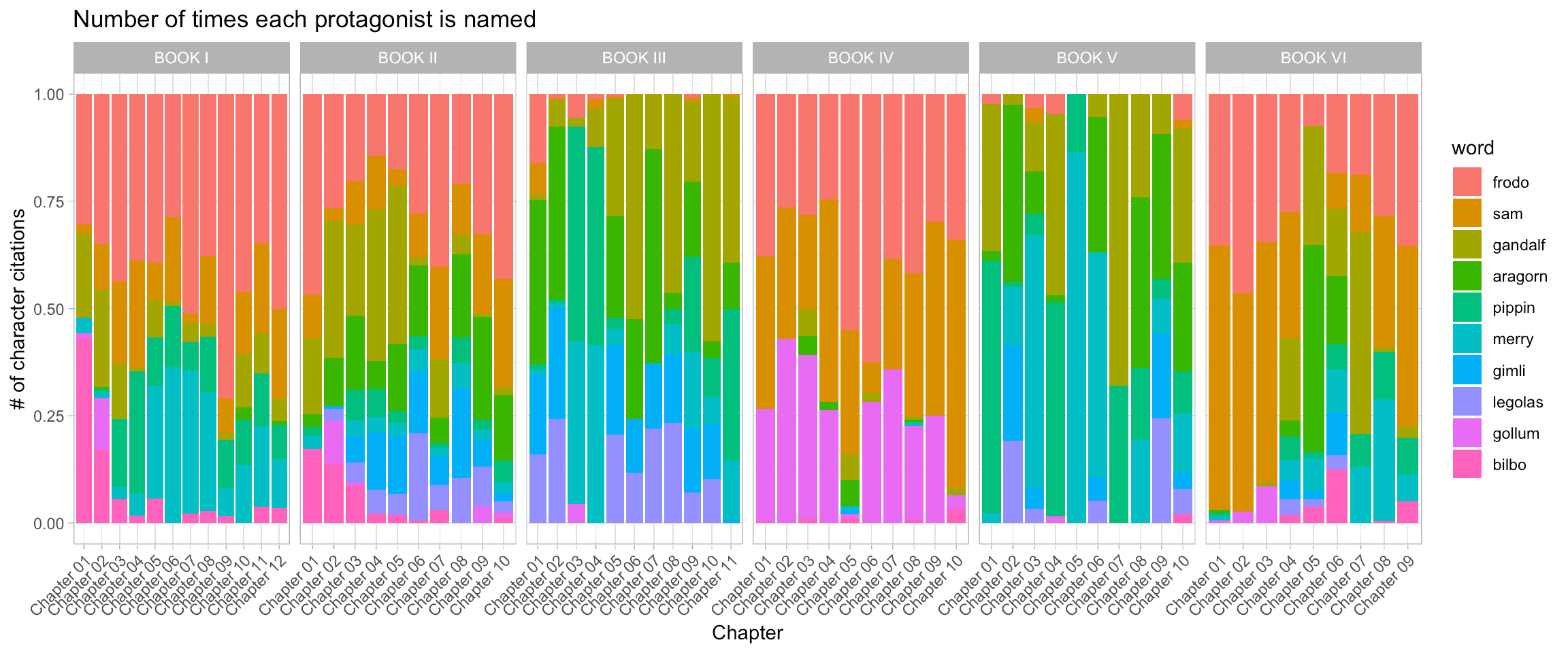
Character networks
TBD
A bit of sentiment analysis
To find the most used non-stop words, one can (1) remove the “stop” words (as defined in the stop_words object), then (2) count the occurence of the remaining words. tidytext and tidyverse are, again, very useful to perform this:
data(stop_words)
top_words <- LOTR %>%
    unnest_tokens(word, text) %>%
    anti_join(stop_words) %>%
    count(book, word, sort = TRUE) %>%
    filter(book %in% "BOOK VI") %>%
    top_n(100) %>%
    pull(word)
## Joining, by = "word"## Selecting by ntop_words## [1] "sam" "frodo" "dark" "merry" "road" "time"
## [7] "looked" "gandalf" "hand" "eyes" "stood" "day"
## [13] "hobbits" "light" "orc" "passed" "black" "king"
## [19] "land" "ring" "left" "days" "folk" "gate"
## [25] "heard" "shire" "west" "set" "night" "tower"
## [31] "master" "pippin" "white" "aragorn" "cried" "round"
## [37] "faramir" "grey" "hope" "mordor" "ran" "ruffians"
## [43] "rode" "water" "fell" "north" "head" "rose"
## [49] "hear" "shadow" "city" "coming" "dead" "hands"
## [55] "voice" "found" "mountain" "fire" "lord" "deep"
## [61] "lay" "door" "drew" "east" "fear" "feet"
## [67] "gondor" "red" "sun" "fair" "heart" "owyn"
## [73] "sat" "wind" "cotton" "lady" "stone" "suddenly"
## [79] "moment" "slowly" "leave" "mind" "people" "darkness"
## [85] "orcs" "saruman" "bag" "bit" "brought" "silver"
## [91] "south" "trees" "walls" "world" "rohan" "wall"
## [97] "chief" "green" "sword" "bilbo" "country" "doom"
## [103] "path" "save"I really like this list of top words. It clearly shows already that there are conflicting feelings in LOTR: we have fear opposing hope, light versus dark, and even temporal contrasts with day and night…
LOTR %>%
    filter(!is.na(chapter) & !is.na(book)) %>%
    unnest_tokens(word, text) %>%
    filter(word %in% top_words) %>%
    mutate(chapter_title = factor(chapter_title, unique(chapter_title))) %>%
    mutate(word = factor(word, top_words)) %>%
    filter(book %in% "BOOK VI") %>%
    count(chapter_title, word) %>%
    ggplot(aes(x = word, y = n)) +
    geom_col() +
    facet_grid(~chapter_title, scales = "free") +
    coord_flip() +
    theme_light() +
    theme(axis.text.x = element_text(angle = 45, hjust = 1, vjust = 1)) +
    labs(x = 'Top words', y = '# of occurences', title = "Number of times each word is mentionned") +
    theme(text = element_text(size = 6))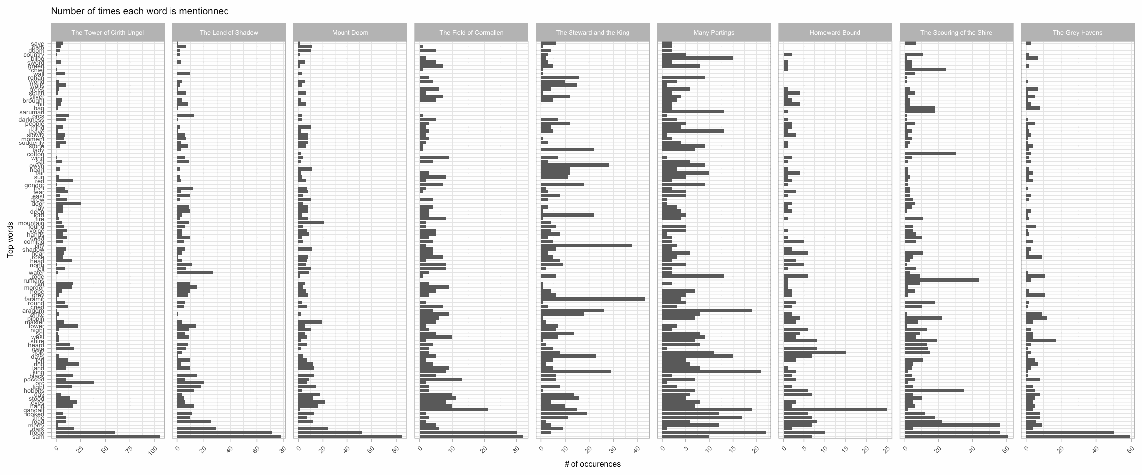
Ideally, one would want to re-organize terms based on how they occur.
words_order <- LOTR %>%
    filter(!is.na(chapter) & !is.na(book)) %>%
    unnest_tokens(word, text) %>%
    filter(word %in% top_words) %>%
    mutate(word = factor(word, top_words)) %>%
    filter(book %in% "BOOK VI") %>%
    count(chapter_title, word) %>%
    spread(word, n) %>%
    column_to_rownames('chapter_title') %>%
    t() %>%
    replace_na(0) %>%
    dist() %>%
    hclust() %$%
    order %>%
    top_words[.]
LOTR %>%
filter(!is.na(chapter) & !is.na(book)) %>%
unnest_tokens(word, text) %>%
filter(word %in% top_words) %>%
mutate(word = factor(word, words_order)) %>%
filter(book %in% "BOOK VI") %>%
count(chapter_title, word) %>%
ggplot(aes(x = word, y = n)) +
geom_col() +
facet_grid(~chapter_title, scales = "free") +
coord_flip() +
theme_light() +
theme(axis.text.x = element_text(angle = 45, hjust = 1, vjust = 1)) +
labs(x = 'Top words', y = '# of occurences', title = "Number of times each word is mentionned") +
theme(text = element_text(size = 6))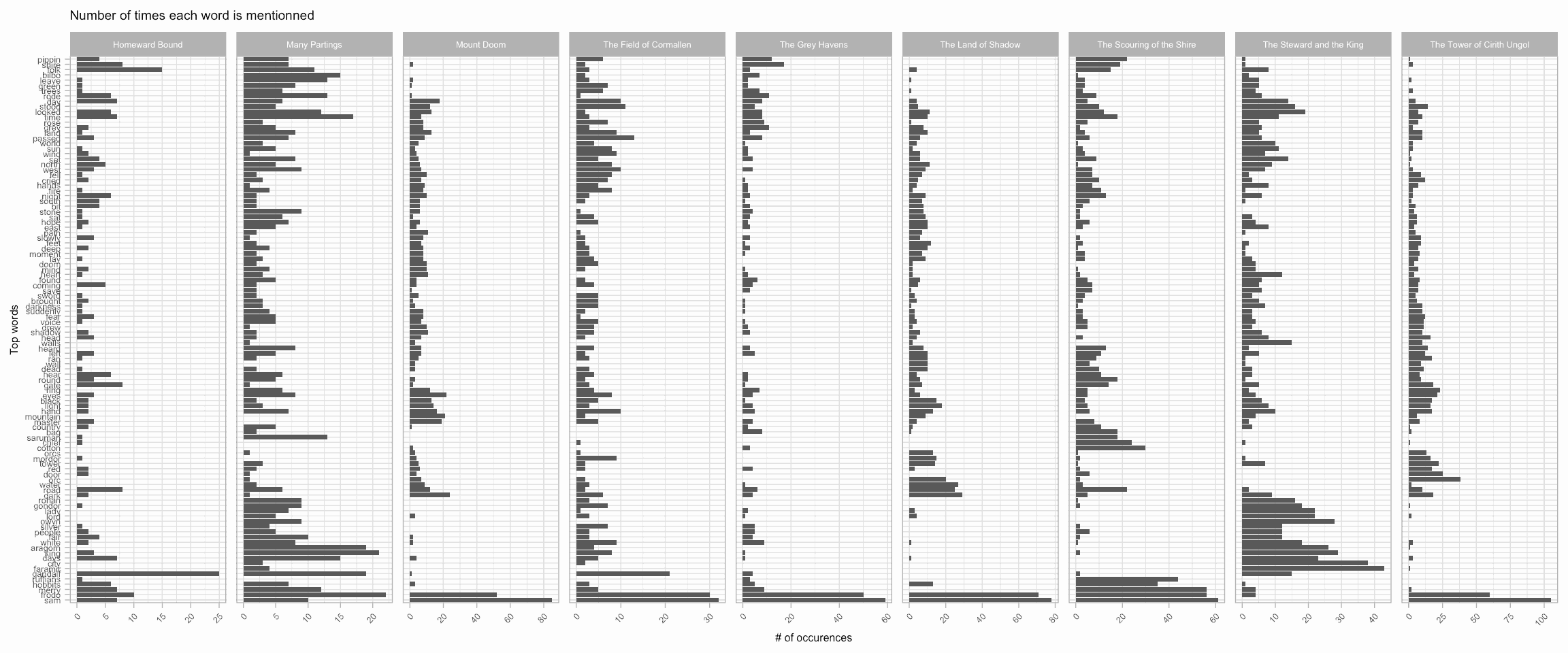
By re-ordering the words, we can clearly see that words describing the hobbits heading back the the Shire are grouped together, while humans returning to the Gondor form another cluster, and orcs and the Mordor in a last separate clique.
Let’s now focus on sentiment analysis. We can get the NRC sentiment lexicon published by Mohammad, Saif M. and Turney, Peter D. in 2013.
sentiment_words <- get_sentiments("nrc")
sentiments <- LOTR %>%
    filter(!is.na(chapter) & !is.na(book)) %>%
    unnest_tokens(word, text) %>%
    group_by(book) %>%
    mutate(progression = as.integer(cut(1:n(), 100))) %>%
    group_by(book, progression) %>%
    inner_join(sentiment_words) %>%
    count(book, sentiment)
## Joining, by = "word"sentiments %>%
filter(sentiment %in% c('positive', 'negative')) %>%
ggplot(aes(x = progression, y = n, fill = sentiment)) +
geom_col() +
facet_grid(book~sentiment, scales = "free") +
theme_light() +
theme(axis.text.x = element_text(angle = 45, hjust = 1, vjust = 1)) +
labs(x = 'Chapter', y = 'Number of occurences', title = 'Number of times a word occurs')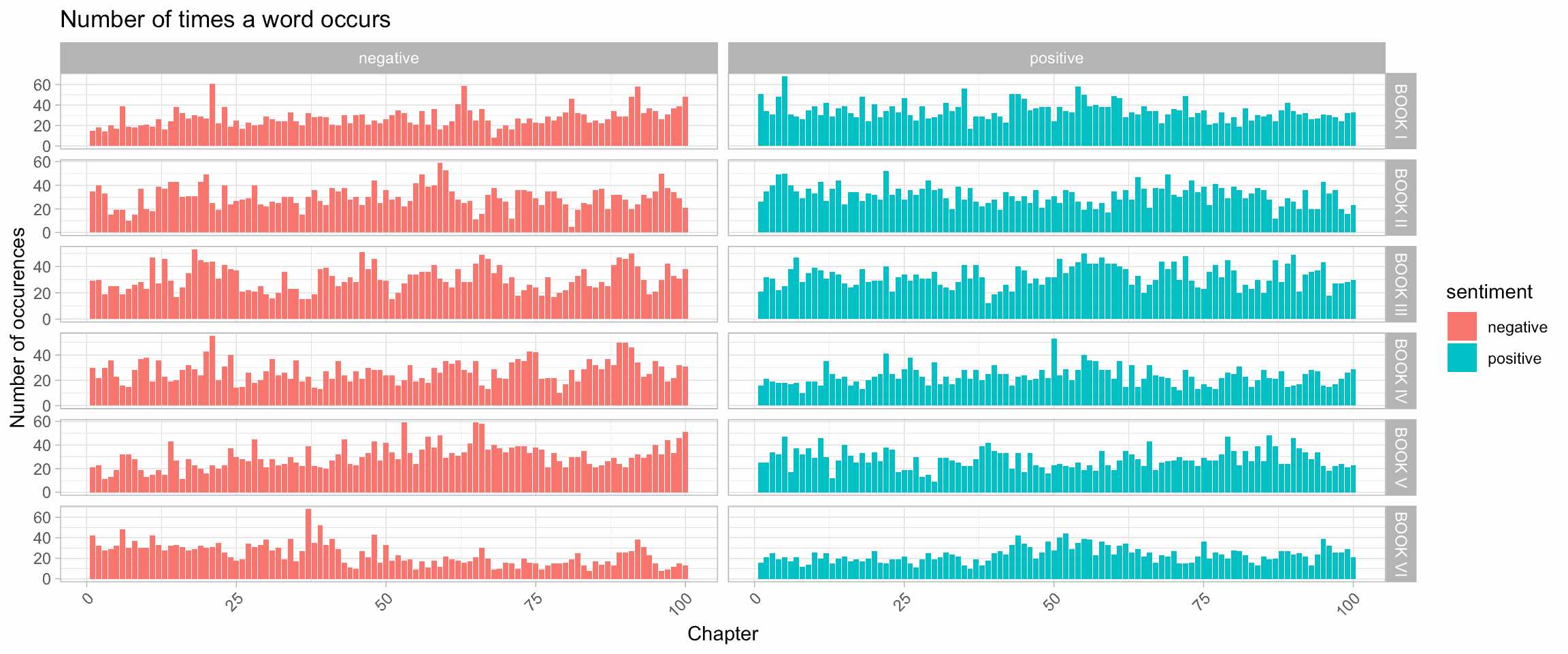
We can focus on Book VI for a bit, with more of the sentiments described by the NCR lexicon:
sentiments_bookVI <- LOTR %>%
    filter(!is.na(chapter) & !is.na(book)) %>%
    unnest_tokens(word, text) %>%
    filter(book == 'BOOK VI') %>%
    mutate(progression = as.integer(cut(1:n(), 100))) %>%
    group_by(progression) %>%
    inner_join(sentiment_words) %>%
    count(sentiment)
## Joining, by = "word"sentiments_bookVI %>%
ggplot(aes(x = progression, y = n, fill = sentiment), col = NA) +
geom_col() +
geom_vline(aes(xintercept = 37), col = 'black', linetype = 'dashed', size = 0.5) +
geom_vline(aes(xintercept = 75), col = 'black', linetype = 'dashed', size = 0.5) +
facet_grid(sentiment~., scales = "free") +
theme_light() +
theme(axis.text.x = element_text(angle = 45, hjust = 1, vjust = 1)) +
labs(x = 'Progression through book VI', y = 'Sentiment score', title = 'Sentiment analysis of Book VI')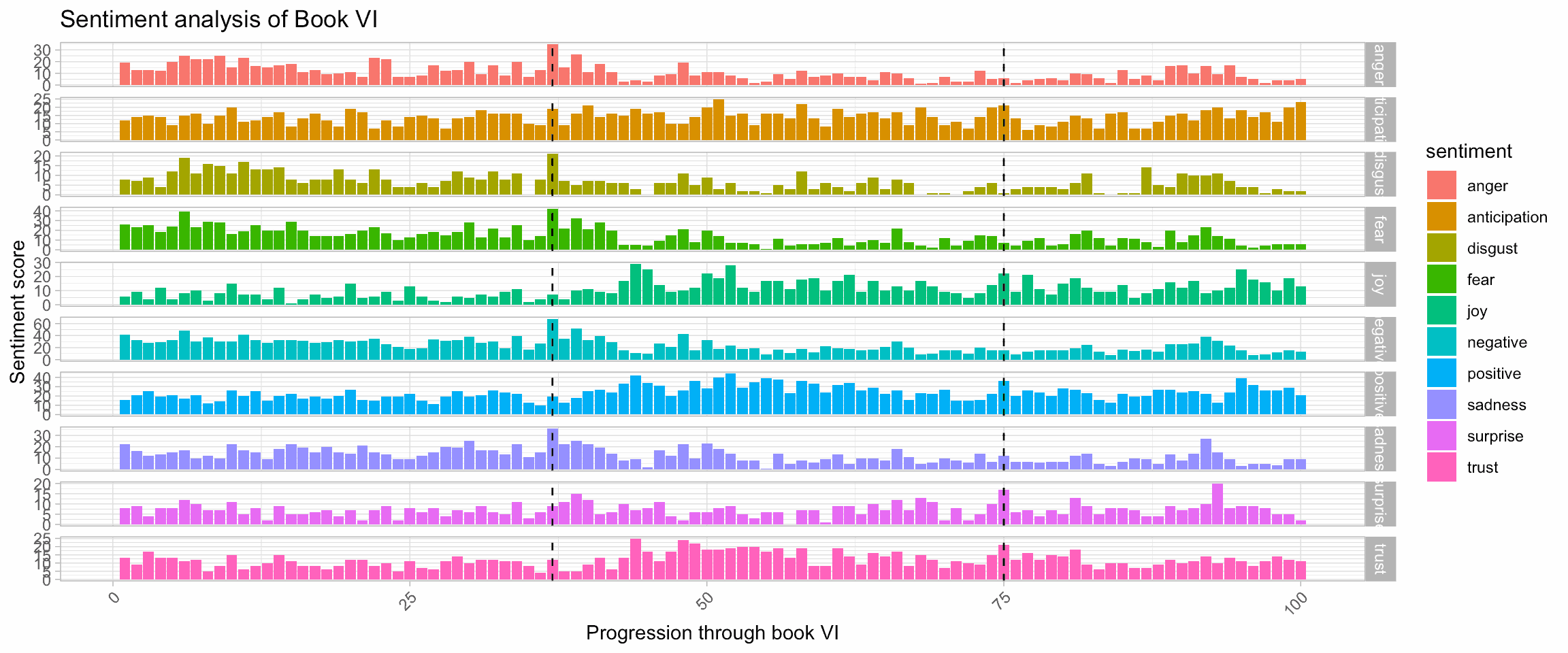
The different sentiments highlight the different key events occuring in the Book VI. For instance:
- At the first third of Book VI: Frodo and Sam reach the Cracks of Doom. It is a pretty dark moment of despair, exhaustion and depression. Yet, it signs the end of all these feelings and the return of hope and joy.
- At the three quarters of Book VI, the Company arrives in Bree and Frodo recalls his long adventures. It is a happy moment with friends gathering in a safe and known place.
Conclusion
This post shows how the tidyverse can be extended to text mining, thanks to the tidytext package. By keeping things tidy, neat analyses and powerful visualization can be obtained very easily, in few lines of code.