Animated plots and single-cell RNA-seq analysis

I know I am probably being over-enthousiastic about it, but I keep learning about ggplot2 features and I can’t get enough of it. Lately, I have discovered the possibilities of animating ggplots based on aesthetics of interest, and as usual, this is as simple as a single line of code…
In this post, I will rely on some single-cell RNA-seq data (from a 10X Genomics sequencing run) containing gene expression for ~500 mouse cycling Radial Glial Progenitors (RGPs).
Loading the single-cell dataset as a SingleCellExperiment object
library(SingleCellExperiment)## Loading required package: SummarizedExperiment## Loading required package: MatrixGenerics## Loading required package: matrixStats##
## Attaching package: 'MatrixGenerics'## The following objects are masked from 'package:matrixStats':
##
## colAlls, colAnyNAs, colAnys, colAvgsPerRowSet, colCollapse,
## colCounts, colCummaxs, colCummins, colCumprods, colCumsums,
## colDiffs, colIQRDiffs, colIQRs, colLogSumExps, colMadDiffs,
## colMads, colMaxs, colMeans2, colMedians, colMins, colOrderStats,
## colProds, colQuantiles, colRanges, colRanks, colSdDiffs, colSds,
## colSums2, colTabulates, colVarDiffs, colVars, colWeightedMads,
## colWeightedMeans, colWeightedMedians, colWeightedSds,
## colWeightedVars, rowAlls, rowAnyNAs, rowAnys, rowAvgsPerColSet,
## rowCollapse, rowCounts, rowCummaxs, rowCummins, rowCumprods,
## rowCumsums, rowDiffs, rowIQRDiffs, rowIQRs, rowLogSumExps,
## rowMadDiffs, rowMads, rowMaxs, rowMeans2, rowMedians, rowMins,
## rowOrderStats, rowProds, rowQuantiles, rowRanges, rowRanks,
## rowSdDiffs, rowSds, rowSums2, rowTabulates, rowVarDiffs, rowVars,
## rowWeightedMads, rowWeightedMeans, rowWeightedMedians,
## rowWeightedSds, rowWeightedVars## Loading required package: GenomicRanges## Loading required package: stats4## Loading required package: BiocGenerics## Loading required package: parallel##
## Attaching package: 'BiocGenerics'## The following objects are masked from 'package:parallel':
##
## clusterApply, clusterApplyLB, clusterCall, clusterEvalQ,
## clusterExport, clusterMap, parApply, parCapply, parLapply,
## parLapplyLB, parRapply, parSapply, parSapplyLB## The following objects are masked from 'package:stats':
##
## IQR, mad, sd, var, xtabs## The following objects are masked from 'package:base':
##
## anyDuplicated, append, as.data.frame, basename, cbind, colnames,
## dirname, do.call, duplicated, eval, evalq, Filter, Find, get, grep,
## grepl, intersect, is.unsorted, lapply, Map, mapply, match, mget,
## order, paste, pmax, pmax.int, pmin, pmin.int, Position, rank,
## rbind, Reduce, rownames, sapply, setdiff, sort, table, tapply,
## union, unique, unsplit, which.max, which.min## Loading required package: S4Vectors##
## Attaching package: 'S4Vectors'## The following object is masked from 'package:base':
##
## expand.grid## Loading required package: IRanges## Loading required package: GenomeInfoDb## Loading required package: Biobase## Welcome to Bioconductor
##
## Vignettes contain introductory material; view with
## 'browseVignettes()'. To cite Bioconductor, see
## 'citation("Biobase")', and for packages 'citation("pkgname")'.##
## Attaching package: 'Biobase'## The following object is masked from 'package:MatrixGenerics':
##
## rowMedians## The following objects are masked from 'package:matrixStats':
##
## anyMissing, rowMedianscyclingCells <- readRDS('data/cyclingCells.rds')
cyclingCells## class: SingleCellExperiment
## dim: 31053 472
## metadata(1): Samples
## assays(2): counts logcounts
## rownames(31053): Xkr4 Gm1992 ... Vmn2r122 CAAA01147332.1
## rowData names(4): ID Symbol mean detected
## colnames: NULL
## colData names(6): Barcode sum ... CellCyclePhase
## pseudotime_velociraptor
## reducedDimNames(0):
## altExpNames(0):head(rowData(cyclingCells))## DataFrame with 6 rows and 4 columns
## ID Symbol mean detected
## <character> <character> <numeric> <numeric>
## Xkr4 ENSMUSG00000051951 Xkr4 0.006024096 0.5733778
## Gm1992 ENSMUSG00000089699 Gm1992 0.000725795 0.0725795
## Gm37381 ENSMUSG00000102343 Gm37381 0.000435477 0.0435477
## Rp1 ENSMUSG00000025900 Rp1 0.029249528 2.4023806
## Sox17 ENSMUSG00000025902 Sox17 0.000000000 0.0000000
## Gm37323 ENSMUSG00000104328 Gm37323 0.001959646 0.1959646head(colData(cyclingCells))## DataFrame with 6 rows and 6 columns
## Barcode sum detected label CellCyclePhase
## <character> <numeric> <integer> <numeric> <factor>
## 1 AAACGAATCCACTGAA-1 18016 5140 15 S
## 2 AAAGAACCATGAAGCG-1 29381 5750 15 G2M
## 3 AAAGAACTCTCGGTCT-1 10394 3484 15 G2M
## 4 AAAGGATCAACCAACT-1 35803 6602 15 G1
## 5 AAAGGATCAATTGCCA-1 27355 5939 15 G2M
## 6 AAAGTGACACTGGATT-1 12503 3739 15 G1
## pseudotime_velociraptor
## <numeric>
## 1 0.131315
## 2 0.155367
## 3 0.168767
## 4 0.396839
## 5 0.199662
## 6 0.260526Embedding cells in lower dimensional space
library(scran)
library(scater)
## Loading required package: ggplot2set.seed(100)
cycling_genes <- c(
"Aurkb", "Ccnb1", "Ccnb2", "Ccnd1", "Ccnd2", "Cdc20", "Cdca3",
"Cdk1", "Cdkn3", "Cenpa", "Cenpe", "Cenpf", "Cenpq", "Cks2",
"Gmnn", "H2afx", "H2afz", "Hist1h1b", "Hist1h1c", "Hist1h1e",
"Hist1h2ae", "Hist1h2bc", "Mcm3", "Mcm4", "Mcm6", "Mki67", "Prc1",
"Serpine2", "Top2a", "Ube2c", "Ube2s"
)
deconv_var <- modelGeneVarByPoisson(cyclingCells)
cyclingCells <- denoisePCA(
cyclingCells,
subset.row = cycling_genes,
technical = deconv_var,
min.rank = 50
)## Warning in check_numbers(k = k, nu = nu, nv = nv, limit = min(dim(x)) - : more
## singular values/vectors requested than available## Warning in (function (A, nv = 5, nu = nv, maxit = 1000, work = nv + 7, reorth =
## TRUE, : You're computing too large a percentage of total singular values, use a
## standard svd instead.## Warning in (function (A, nv = 5, nu = nv, maxit = 1000, work = nv + 7, reorth
## = TRUE, : did not converge--results might be invalid!; try increasing work or
## maxitreducedDim(cyclingCells, "force") <- igraph::layout_with_fr(
buildSNNGraph(
cyclingCells,
use.dimred = "PCA",
subset.row = cycling_genes
)
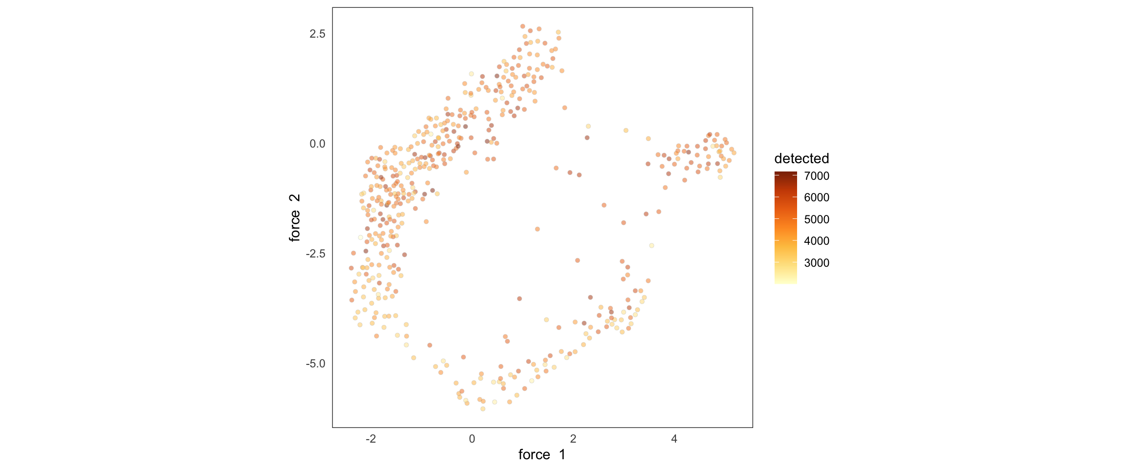
)We can plot the cells embedded in a lower dimensional space with a function from my package of single-cell utilities:
library(SCTools)
# ----- Plotting embedding in a lower dim. space ----- #
SCTools::plotEmbedding(
    cyclingCells,
    "detected",
    "force"
)
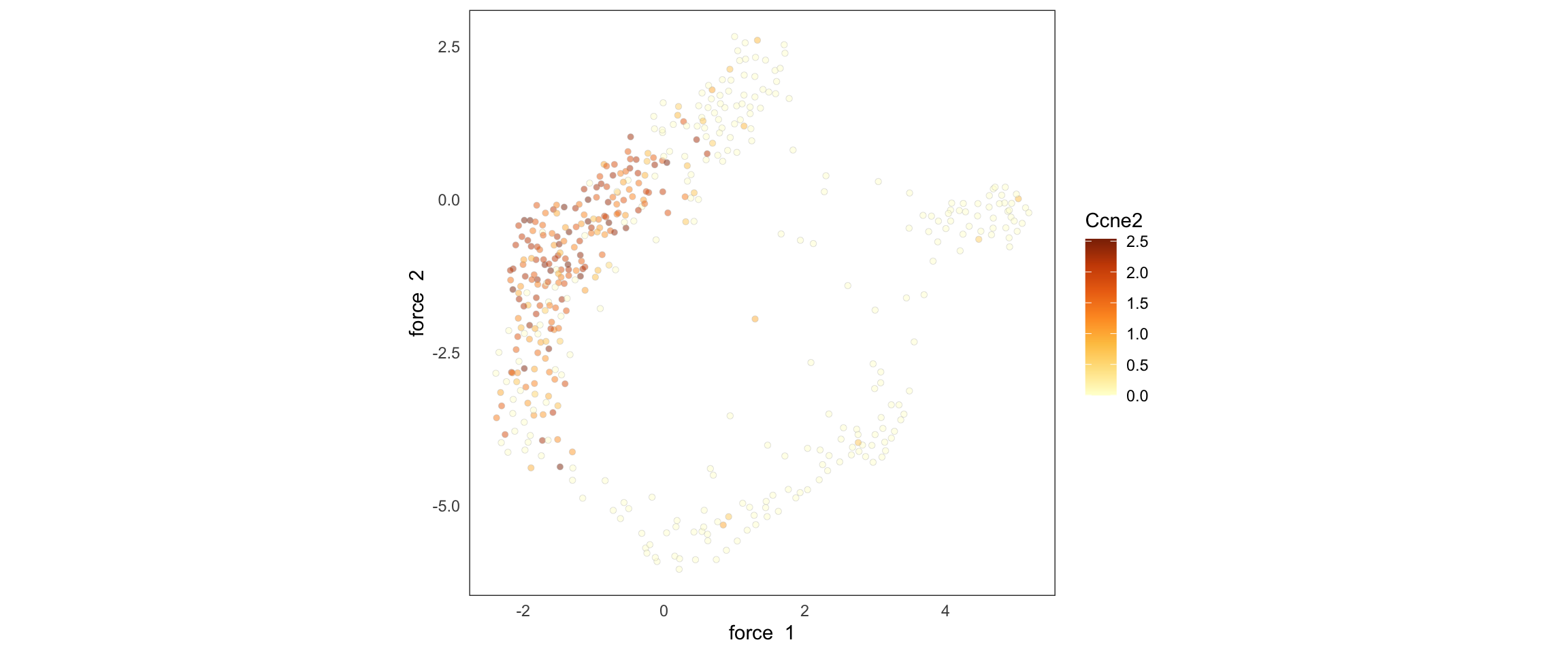
We can also color by levels of gene expression:
SCTools::plotEmbedding(
    cyclingCells,
    "Ccne2",
    "force"
)
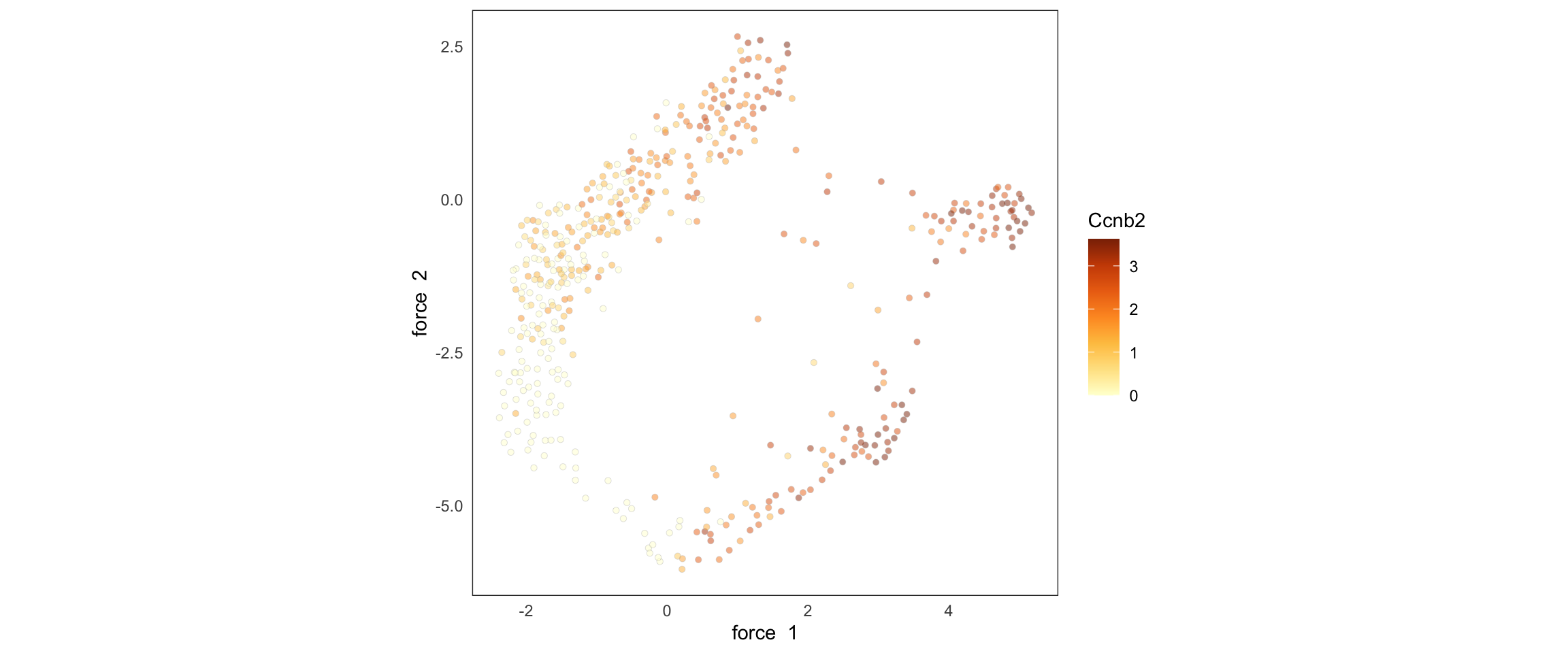
SCTools::plotEmbedding(
    cyclingCells,
    "Ccnb2",
    "force"
)
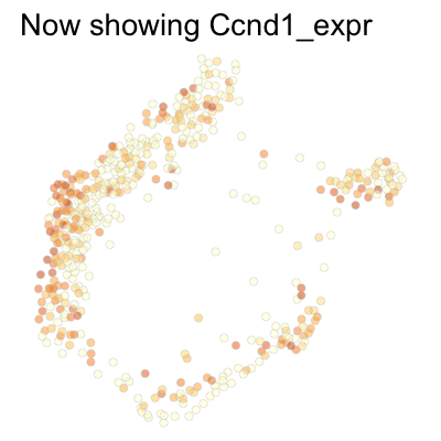
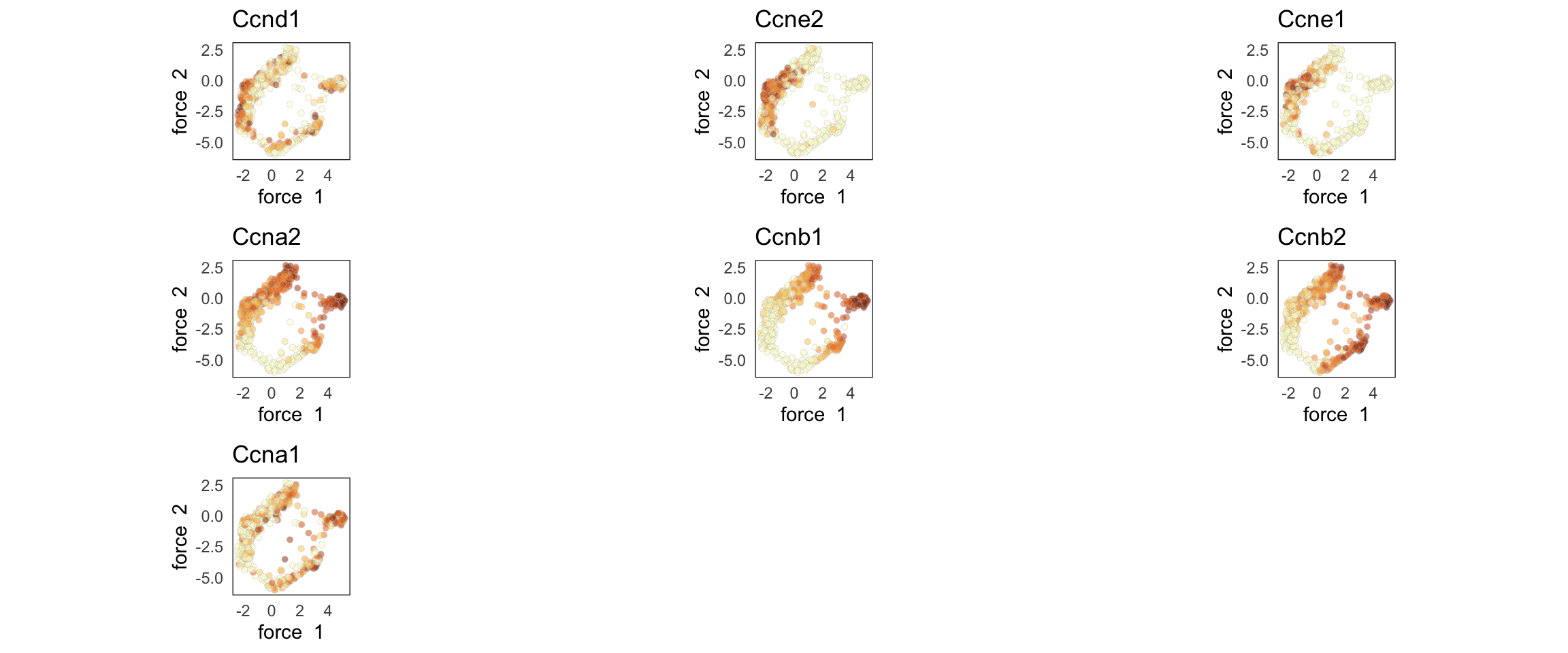
Finally, we can plot several genes at once:
genes <- c('Ccnd1', 'Ccne2', 'Ccne1', 'Ccna2', 'Ccnb1', 'Ccnb2', 'Ccna1')
SCTools::plotEmbedding(
    cyclingCells,
    c('Ccnd1', 'Ccne2', 'Ccne1', 'Ccna2', 'Ccnb1', 'Ccnb2', 'Ccna1'),
    "force",
    theme.args = theme(legend.position = 'none')
)
Putting all these plots in 1 GIF
library(tidyverse)## ── Attaching packages ───────────────────────────────────────────────────────────────────────────────────────────────────────────────────────────────────────────────────────────────────────────────────────────────────────────────────── tidyverse 1.3.0 ──## ✔ tibble 3.0.5 ✔ dplyr 1.0.3
## ✔ tidyr 1.1.2 ✔ stringr 1.4.0
## ✔ readr 1.4.0 ✔ forcats 0.5.0
## ✔ purrr 0.3.4## ── Conflicts ──────────────────────────────────────────────────────────────────────────────────────────────────────────────────────────────────────────────────────────────────────────────────────────────────────────────────────── tidyverse_conflicts() ──
## ✖ dplyr::collapse() masks IRanges::collapse()
## ✖ dplyr::combine() masks Biobase::combine(), BiocGenerics::combine()
## ✖ dplyr::count() masks matrixStats::count()
## ✖ dplyr::desc() masks IRanges::desc()
## ✖ tidyr::expand() masks S4Vectors::expand()
## ✖ dplyr::filter() masks stats::filter()
## ✖ dplyr::first() masks S4Vectors::first()
## ✖ dplyr::lag() masks stats::lag()
## ✖ ggplot2::Position() masks BiocGenerics::Position(), base::Position()
## ✖ purrr::reduce() masks GenomicRanges::reduce(), IRanges::reduce()
## ✖ dplyr::rename() masks S4Vectors::rename()
## ✖ dplyr::slice() masks IRanges::slice()library(magrittr)##
## Attaching package: 'magrittr'## The following object is masked from 'package:purrr':
##
## set_names## The following object is masked from 'package:tidyr':
##
## extractdf <- data.frame(cell = cyclingCells$Barcode)
for (gene in genes) {
expr <- logcounts(cyclingCells)[gene, ] %>% bindByQuantiles(q_low = 0.05, q_high = 0.95)
df[, paste0(gene, "_expr")] <- expr
}
df %<>%
mutate(
X = reducedDim(cyclingCells, 'force')[, 1],
Y = reducedDim(cyclingCells, 'force')[, 2]
) %>%
gather("gene", "expr", -cell, -X, -Y) %>%
mutate(gene = factor(gene, levels = paste0(genes, "_expr"))) %>%
select(X, Y, gene, expr)
head(df)## X Y gene expr
## 1 -1.4996544 -1.3584288 Ccnd1_expr 0.000000
## 2 1.0808325 1.3022992 Ccnd1_expr 0.000000
## 3 0.6696466 1.6447031 Ccnd1_expr 0.000000
## 4 -1.3375422 -2.5331948 Ccnd1_expr 0.000000
## 5 4.3305936 -0.4361058 Ccnd1_expr 2.847585
## 6 -1.9770603 -4.0901018 Ccnd1_expr 0.000000p <- ggplot(df, aes_string(x = "X", y = "Y", fill = "expr")) +
geom_point(pch = 21, alpha = 0.5, col = '#bcbcbc', stroke = 0.2) +
theme_void() + theme(legend.position = 'none') +
scale_fill_distiller(palette = 'YlOrBr', direction = 1) +
coord_fixed((max(df[, "X"])-min(df[, "X"]))/(max(df[, "Y"])-min(df[, "Y"]))) +
labs(y = "force 2", x = "force 1", fill = '') +
theme(
panel.grid.major = element_blank(),
panel.grid.minor = element_blank(),
axis.ticks = element_blank()
) +
gganimate::transition_states(
gene,
transition_length = 1,
state_length = 1
)All of this is actually wrapped into a single function in SCTools:
genes <- c('Ccnd1', 'Ccne2', 'Ccne1', 'Ccna2', 'Ccnb1', 'Ccnb2', 'Ccna1')
colData(cyclingCells)$force_X <- reducedDim(cyclingCells, 'force')[, 1]
colData(cyclingCells)$force_Y <- reducedDim(cyclingCells, 'force')[, 2]
gif <- plotAnimatedEmbedding(
    cyclingCells,
    dim = "force",
    genes = genes,
    theme.args = theme_void() + theme(legend.position = 'none')
) %>% gganimate::animate(
    duration = 2, fps = 20,
    width = 400, height = 400, res = 150,
    renderer = gganimate::gifski_renderer()
)
## Rendering [=====>---------------------------------------] at 23 fps ~ eta: 2s
## Rendering [======>--------------------------------------] at 23 fps ~ eta: 2s
## Rendering [=======>-------------------------------------] at 23 fps ~ eta: 1s
## Rendering [========>------------------------------------] at 23 fps ~ eta: 1s
## Rendering [=========>-----------------------------------] at 23 fps ~ eta: 1s
## Rendering [==========>----------------------------------] at 23 fps ~ eta: 1s
## Rendering [===========>---------------------------------] at 22 fps ~ eta: 1s
## Rendering [=============>-------------------------------] at 22 fps ~ eta: 1s
## Rendering [==============>------------------------------] at 22 fps ~ eta: 1s
## Rendering [===============>-----------------------------] at 22 fps ~ eta: 1s
## Rendering [================>----------------------------] at 22 fps ~ eta: 1s
## Rendering [=================>---------------------------] at 21 fps ~ eta: 1s
## Rendering [==================>--------------------------] at 22 fps ~ eta: 1s
## Rendering [===================>-------------------------] at 22 fps ~ eta: 1s
## Rendering [====================>------------------------] at 21 fps ~ eta: 1s
## Rendering [=====================>-----------------------] at 21 fps ~ eta: 1s
## Rendering [=======================>---------------------] at 22 fps ~ eta: 1s
## Rendering [========================>--------------------] at 21 fps ~ eta: 1s
## Rendering [=========================>-------------------] at 21 fps ~ eta: 1s
## Rendering [==========================>------------------] at 22 fps ~ eta: 1s
## Rendering [===========================>-----------------] at 22 fps ~ eta: 1s
## Rendering [============================>----------------] at 22 fps ~ eta: 1s
## Rendering [=============================>---------------] at 21 fps ~ eta: 1s
## Rendering [==============================>--------------] at 21 fps ~ eta: 1s
## Rendering [================================>------------] at 21 fps ~ eta: 1s
## Rendering [=================================>-----------] at 21 fps ~ eta: 0s
## Rendering [==================================>----------] at 21 fps ~ eta: 0s
## Rendering [===================================>---------] at 21 fps ~ eta: 0s
## Rendering [====================================>--------] at 21 fps ~ eta: 0s
## Rendering [=====================================>-------] at 21 fps ~ eta: 0s
## Rendering [======================================>------] at 21 fps ~ eta: 0s
## Rendering [=======================================>-----] at 21 fps ~ eta: 0s
## Rendering [=========================================>---] at 21 fps ~ eta: 0s
## Rendering [==========================================>--] at 21 fps ~ eta: 0s
## Rendering [===========================================>-] at 21 fps ~ eta: 0s
## Rendering [=============================================] at 21 fps ~ eta: 0sgif