Why is Bioconductor awesome

I love Bioconductor
Since its early ages, Bioconductor has gone very far. I’ve been on board for the past 7-ish years (I think), I use it every day, and every day, I think about how much I love it.
Some reasons…
I love Bioconductor for many reasons, some of them being GenomicRanges, SummarizedExperiment, DESeq2, and of course the amazing team.
But today, one reason which I want to discuss in more depth is the Annotation Hub. This hub provides access to tons of resources, particularly if you work in human genomics. One reason why it’s so useful in human is because major consortia like Encode and Roadmap Epigenomics Project put their data there. So you end up with tons of stuff available, if you know what you are looking for!
An example: finding genes undergoing chromatin state transition during cell differentiation
The Roadmap Epigenomics Project (REP) has characterized chromatin states in tens of epigenomes (that’s literally the title of their paper: Integrative analysis of 111 reference human epigenomes!).
And guess what, all the results are available in the AnnotationHub! Here is a glimpse at some of the data hosted there:
library(tidyverse)## ── Attaching packages ───────────────────────────────────────────────────────────────────────────────────────────────────────────────────────────────────────────────────────────────────────────────────────────────────────────────────── tidyverse 1.3.0 ──## ✔ ggplot2 3.3.3 ✔ purrr 0.3.4
## ✔ tibble 3.0.5 ✔ dplyr 1.0.3
## ✔ tidyr 1.1.2 ✔ stringr 1.4.0
## ✔ readr 1.4.0 ✔ forcats 0.5.0## ── Conflicts ──────────────────────────────────────────────────────────────────────────────────────────────────────────────────────────────────────────────────────────────────────────────────────────────────────────────────────── tidyverse_conflicts() ──
## ✖ dplyr::filter() masks stats::filter()
## ✖ dplyr::lag() masks stats::lag()library(AnnotationHub)## Loading required package: BiocGenerics## Loading required package: parallel##
## Attaching package: 'BiocGenerics'## The following objects are masked from 'package:parallel':
##
## clusterApply, clusterApplyLB, clusterCall, clusterEvalQ,
## clusterExport, clusterMap, parApply, parCapply, parLapply,
## parLapplyLB, parRapply, parSapply, parSapplyLB## The following objects are masked from 'package:dplyr':
##
## combine, intersect, setdiff, union## The following objects are masked from 'package:stats':
##
## IQR, mad, sd, var, xtabs## The following objects are masked from 'package:base':
##
## anyDuplicated, append, as.data.frame, basename, cbind, colnames,
## dirname, do.call, duplicated, eval, evalq, Filter, Find, get, grep,
## grepl, intersect, is.unsorted, lapply, Map, mapply, match, mget,
## order, paste, pmax, pmax.int, pmin, pmin.int, Position, rank,
## rbind, Reduce, rownames, sapply, setdiff, sort, table, tapply,
## union, unique, unsplit, which.max, which.min## Loading required package: BiocFileCache## Loading required package: dbplyr##
## Attaching package: 'dbplyr'## The following objects are masked from 'package:dplyr':
##
## ident, sqlah <- AnnotationHub()## using temporary cache /var/folders/qm/3bz0g1zn5wnb9ck9_lfwhpcm0000gn/T//RtmpGrlDwB/BiocFileCache## snapshotDate(): 2020-10-27ah_human_epigenome <- query(ah, c("Homo sapiens", "EpigenomeRoadMap"))
table(ah_human_epigenome$rdataclass)##
## BigWigFile data.frame GRanges
## 9932 15 8301head(query(ah_human_epigenome, 'BigWigFile')$title, 50)## [1] "E001-H3K4me1.fc.signal.bigwig" "E001-H3K4me3.fc.signal.bigwig"
## [3] "E001-H3K9ac.fc.signal.bigwig" "E001-H3K9me3.fc.signal.bigwig"
## [5] "E001-H3K27me3.fc.signal.bigwig" "E001-H3K36me3.fc.signal.bigwig"
## [7] "E002-H3K4me1.fc.signal.bigwig" "E002-H3K4me3.fc.signal.bigwig"
## [9] "E002-H3K9ac.fc.signal.bigwig" "E002-H3K9me3.fc.signal.bigwig"
## [11] "E002-H3K27me3.fc.signal.bigwig" "E002-H3K36me3.fc.signal.bigwig"
## [13] "E003-DNase.fc.signal.bigwig" "E003-H2A.Z.fc.signal.bigwig"
## [15] "E003-H2AK5ac.fc.signal.bigwig" "E003-H2BK5ac.fc.signal.bigwig"
## [17] "E003-H2BK12ac.fc.signal.bigwig" "E003-H2BK15ac.fc.signal.bigwig"
## [19] "E003-H2BK20ac.fc.signal.bigwig" "E003-H2BK120ac.fc.signal.bigwig"
## [21] "E003-H3K4ac.fc.signal.bigwig" "E003-H3K4me1.fc.signal.bigwig"
## [23] "E003-H3K4me2.fc.signal.bigwig" "E003-H3K4me3.fc.signal.bigwig"
## [25] "E003-H3K9ac.fc.signal.bigwig" "E003-H3K9me3.fc.signal.bigwig"
## [27] "E003-H3K14ac.fc.signal.bigwig" "E003-H3K18ac.fc.signal.bigwig"
## [29] "E003-H3K23ac.fc.signal.bigwig" "E003-H3K23me2.fc.signal.bigwig"
## [31] "E003-H3K27ac.fc.signal.bigwig" "E003-H3K27me3.fc.signal.bigwig"
## [33] "E003-H3K36me3.fc.signal.bigwig" "E003-H3K56ac.fc.signal.bigwig"
## [35] "E003-H3K79me1.fc.signal.bigwig" "E003-H3K79me2.fc.signal.bigwig"
## [37] "E003-H4K5ac.fc.signal.bigwig" "E003-H4K8ac.fc.signal.bigwig"
## [39] "E003-H4K20me1.fc.signal.bigwig" "E003-H4K91ac.fc.signal.bigwig"
## [41] "E004-DNase.fc.signal.bigwig" "E004-H2AK5ac.fc.signal.bigwig"
## [43] "E004-H2BK5ac.fc.signal.bigwig" "E004-H2BK15ac.fc.signal.bigwig"
## [45] "E004-H2BK120ac.fc.signal.bigwig" "E004-H3K4ac.fc.signal.bigwig"
## [47] "E004-H3K4me1.fc.signal.bigwig" "E004-H3K4me2.fc.signal.bigwig"
## [49] "E004-H3K4me3.fc.signal.bigwig" "E004-H3K9ac.fc.signal.bigwig"Wow, almost 10K of bigwig files. Neat!
What about metadata? It is available in the accession AH41830.
epigenome_metadata <- ah_human_epigenome[['AH41830']]## downloading 1 resources## retrieving 1 resource## loading from cacheepigenome_metadata[1:10, 1:10]## EID GROUP COLOR MNEMONIC
## 1 E001 ESC #924965 ESC.I3
## 2 E002 ESC #924965 ESC.WA7
## 3 E003 ESC #924965 ESC.H1
## 4 E004 ES-deriv #4178AE ESDR.H1.BMP4.MESO
## 5 E005 ES-deriv #4178AE ESDR.H1.BMP4.TROP
## 6 E006 ES-deriv #4178AE ESDR.H1.MSC
## 7 E007 ES-deriv #4178AE ESDR.H1.NEUR.PROG
## 8 E008 ESC #924965 ESC.H9
## 9 E009 ES-deriv #4178AE ESDR.H9.NEUR.PROG
## 10 E010 ES-deriv #4178AE ESDR.H9.NEUR
## STD_NAME
## 1 ES-I3 Cells
## 2 ES-WA7 Cells
## 3 H1 Cells
## 4 H1 BMP4 Derived Mesendoderm Cultured Cells
## 5 H1 BMP4 Derived Trophoblast Cultured Cells
## 6 H1 Derived Mesenchymal Stem Cells
## 7 H1 Derived Neuronal Progenitor Cultured Cells
## 8 H9 Cells
## 9 H9 Derived Neuronal Progenitor Cultured Cells
## 10 H9 Derived Neuron Cultured Cells
## EDACC_NAME ANATOMY TYPE AGE
## 1 ES-I3_Cell_Line ESC PrimaryCulture CL
## 2 ES-WA7_Cell_Line ESC PrimaryCulture CL
## 3 H1_Cell_Line ESC PrimaryCulture CL
## 4 H1_BMP4_Derived_Mesendoderm_Cultured_Cells ESC_DERIVED ESCDerived CL
## 5 H1_BMP4_Derived_Trophoblast_Cultured_Cells ESC_DERIVED ESCDerived CL
## 6 H1_Derived_Mesenchymal_Stem_Cells ESC_DERIVED ESCDerived CL
## 7 H1_Derived_Neuronal_Progenitor_Cultured_Cells ESC_DERIVED ESCDerived CL
## 8 H9_Cell_Line ESC PrimaryCulture CL
## 9 H9_Derived_Neuronal_Progenitor_Cultured_Cells ESC_DERIVED ESCDerived CL
## 10 H9_Derived_Neuron_Cultured_Cells ESC_DERIVED ESCDerived CL
## SEX
## 1 Female
## 2 Female
## 3 Male
## 4 Male
## 5 Male
## 6 Male
## 7 Male
## 8 Female
## 9 Female
## 10 FemaleCool. Next, we are going to focus on chromatin state segmentation. What’s available there?
query(ah_human_epigenome, c("chromhmmSegmentations", "cell line"))## AnnotationHub with 5 records
## # snapshotDate(): 2020-10-27
## # $dataprovider: BroadInstitute
## # $species: Homo sapiens
## # $rdataclass: GRanges
## # additional mcols(): taxonomyid, genome, description,
## # coordinate_1_based, maintainer, rdatadateadded, preparerclass, tags,
## # rdatapath, sourceurl, sourcetype
## # retrieve records with, e.g., 'object[["AH46872"]]'
##
## title
## AH46872 | E017_15_coreMarks_mnemonics.bed.gz
## AH46967 | E114_15_coreMarks_mnemonics.bed.gz
## AH46968 | E115_15_coreMarks_mnemonics.bed.gz
## AH46970 | E117_15_coreMarks_mnemonics.bed.gz
## AH46971 | E118_15_coreMarks_mnemonics.bed.gzLooks like 5 different epigenomes were segmented into chromatin states. The ones that we are interested in are those from H1 embryonic stem cells (H1) or from Neural Progenitor Cells (NPCs) derived from these H1 cells.
H1_states <- query(ah_human_epigenome, c("chromhmmSegmentations", "ESC.H1"))[[1]]## downloading 1 resources## retrieving 1 resource## loading from cache## require("rtracklayer")NPC_states <- query(ah_human_epigenome, c("chromhmmSegmentations", "ESDR.H1.NEUR.PROG"))[[1]]## downloading 1 resources## retrieving 1 resource## loading from cacheH1_states <- resize(H1_states, 1, fix = 'center') # Resizing to make it easier to find overlaps
NPC_states <- resize(NPC_states, 1, fix = 'center') # Resizing to make it easier to find overlapsLet’s find out how loci are changing between H1 and NPC cultures:
states <- c(
    "Active TSS",
    "Flanking Active TSS",
    "Bivalent/Poised TSS",
    "Enhancers",
    "Flanking Bivalent TSS/Enh",
    "Strong transcription",
    "Transcr. at gene 5' and 3'",
    "Weak transcription",
    "Bivalent Enhancer",
    "Genic enhancers",
    "Quiescent/Low",
    "Heterochromatin",
    "Weak Repressed PolyComb",
    "Repressed PolyComb",
    "ZNF genes & repeats"
)
df <- data.frame(
    stateInH1 = factor(H1_states$name, levels = states),
    stateInNPCs = factor(NPC_states[nearest(H1_states, NPC_states)]$name, levels = states)
)
df %>%
    group_by(stateInH1, stateInNPCs) %>%
    summarize(count = n()) %>%
    mutate(label = ifelse(count > 1000, count, '')) %>%
    ggplot(aes(x = stateInH1, y = stateInNPCs, fill = count, label = label)) +
    geom_tile(col = "black") +
    geom_text(size = 1.5) +
    theme_bw() +
    scale_fill_gradientn(colours = c('white', 'orange', 'darkred')) +
    theme(
        axis.text.x = element_text(angle = 90, hjust = 1, vjust = 0.5),
        panel.border = element_blank(),
        panel.grid.major = element_blank(),
        panel.grid.minor = element_blank(),
        axis.ticks = element_blank()
    ) +
    labs(
        x = "Chromatin states in H1 cells",
        y = "Chromatin states in H1-derived\nneural progenitor cells",
        fill = '#'
    ) +
    coord_fixed()
## `summarise()` has grouped output by 'stateInH1'. You can override using the `.groups` argument.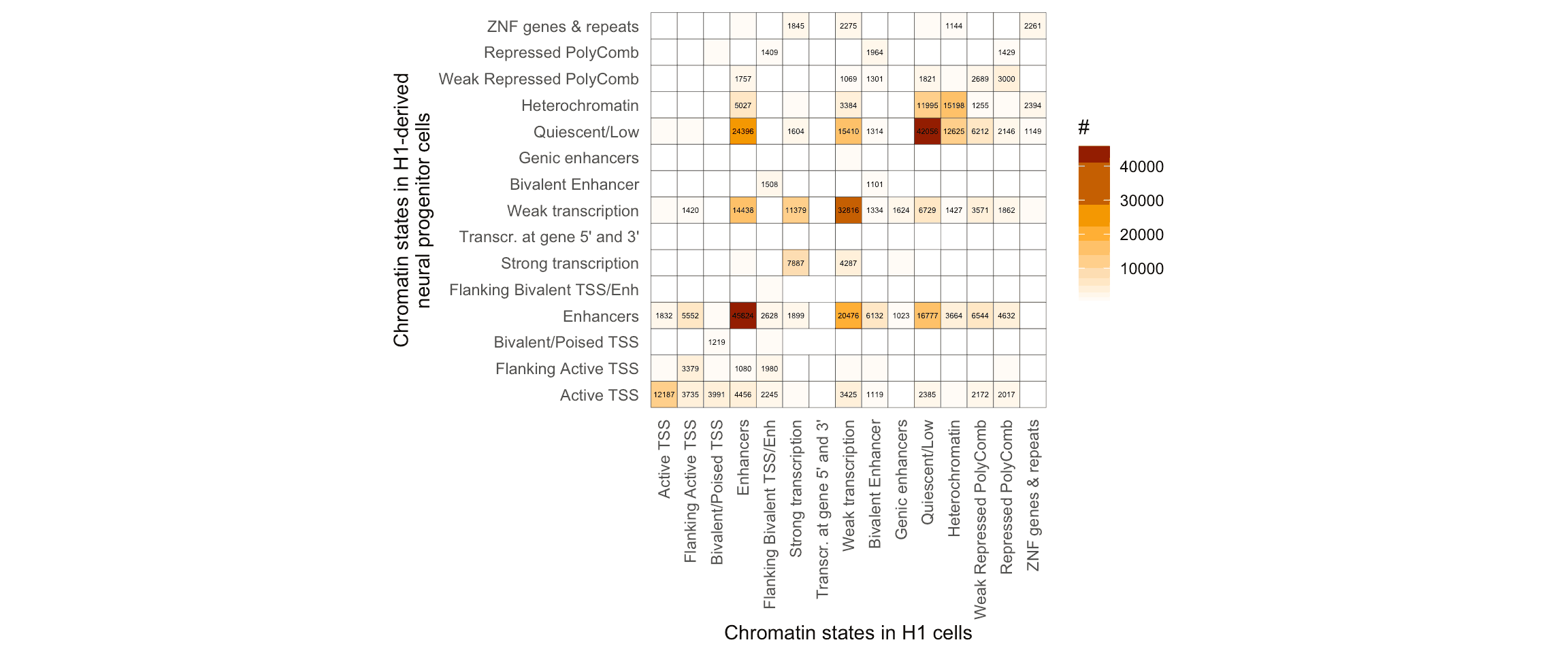
Using the tidyverse to plot the transitions, it’s clear that while most of the segmented genomic loci keep their functional annotation from ESCs to NPCs, there are other loci which change from inactive to activate chromatin states, and vice versa.
For instance, let’s focus on the loci undergoing changes from a Repressed PolyComb state to a Enhancers state:
transitioning_loci <- H1_states[df$stateInH1 == 'Repressed PolyComb' & df$stateInNPCs == 'Enhancers']
transitioning_loci
## GRanges object with 4632 ranges and 4 metadata columns:
## seqnames ranges strand | abbr name color_name
## <Rle> <IRanges> <Rle> | <character> <character> <character>
## [1] chr10 552700 * | 13_ReprPC Repressed PolyComb Silver
## [2] chr10 654300 * | 13_ReprPC Repressed PolyComb Silver
## [3] chr10 1782600 * | 13_ReprPC Repressed PolyComb Silver
## [4] chr10 5725500 * | 13_ReprPC Repressed PolyComb Silver
## [5] chr10 6185700 * | 13_ReprPC Repressed PolyComb Silver
## ... ... ... ... . ... ... ...
## [4628] chrX 154027500 * | 13_ReprPC Repressed PolyComb Silver
## [4629] chrX 154029600 * | 13_ReprPC Repressed PolyComb Silver
## [4630] chrY 6758600 * | 13_ReprPC Repressed PolyComb Silver
## [4631] chrY 6761100 * | 13_ReprPC Repressed PolyComb Silver
## [4632] chrY 6765700 * | 13_ReprPC Repressed PolyComb Silver
## color_code
## <character>
## [1] #808080
## [2] #808080
## [3] #808080
## [4] #808080
## [5] #808080
## ... ...
## [4628] #808080
## [4629] #808080
## [4630] #808080
## [4631] #808080
## [4632] #808080
## -------
## seqinfo: 298 sequences (2 circular) from hg19 genomeNow, let’s fetch the genes associated to these loci. This is easily done, again, by retrieving informatin from AnnotationHub!
I will retrieve the human gene model from AnnotationHub:
human_gtf <- query(ah, c("Homo sapiens", "release-75"))[[1]]## downloading 1 resources## retrieving 1 resource## loading from cacheseqlevelsStyle(human_gtf) <- "UCSC"
human_gtf <- keepStandardChromosomes(human_gtf, pruning.mode = 'coarse')
human_genes <- human_gtf[human_gtf$type == 'gene' & human_gtf$gene_biotype == 'protein_coding']
human_TSSs <- resize(human_genes, 1, 'start')I can then retrieve the closest gene for each of the transitioning loci, and filter the genes that are close to these transitioning loci.
transitioning_loci$nearest_gene <- human_TSSs[nearest(transitioning_loci, human_TSSs)]$gene_id
transitioning_loci$distance_to_nearest_gene <- mcols(distanceToNearest(transitioning_loci, human_TSSs))$distance
genes <- unique(transitioning_loci$nearest_gene[transitioning_loci$distance_to_nearest_gene <= 1000])
Finally, a quick GO over-representation analysis will reveal whether these few genes are indeed involved in any neural process. Once again, I can retrieve ontology from human OrgDb using AnnotationHub:
org <- query(ah, c('homo sapiens', 'orgdb'))[[1]]## downloading 1 resources## retrieving 1 resource## loading from cache## Loading required package: AnnotationDbi## Loading required package: Biobase## Welcome to Bioconductor
##
## Vignettes contain introductory material; view with
## 'browseVignettes()'. To cite Bioconductor, see
## 'citation("Biobase")', and for packages 'citation("pkgname")'.##
## Attaching package: 'Biobase'## The following object is masked from 'package:AnnotationHub':
##
## cache##
## Attaching package: 'AnnotationDbi'## The following object is masked from 'package:dplyr':
##
## selectres <- clusterProfiler::enrichGO(
genes,
OrgDb = org,
ont = 'CC',
keyType = 'ENSEMBL',
pvalueCutoff = 0.05,
qvalueCutoff = 0.05
)## res@result %>% dplyr::select(Description, pvalue, p.adjust, Count) %>% arrange(p.adjust) %>% filter(p.adjust < 0.05)## Description pvalue p.adjust
## GO:0031256 leading edge membrane 5.725696e-05 0.01691181
## GO:0032590 dendrite membrane 1.218905e-04 0.01691181
## GO:0098978 glutamatergic synapse 1.666276e-04 0.01691181
## GO:0045211 postsynaptic membrane 2.081453e-04 0.01691181
## GO:0097060 synaptic membrane 3.054852e-04 0.01792994
## GO:0150034 distal axon 3.310143e-04 0.01792994
## GO:0044306 neuron projection terminus 4.010680e-04 0.01862101
## GO:0043195 terminal bouton 5.914433e-04 0.02143279
## GO:0099699 integral component of synaptic membrane 6.319324e-04 0.02143279
## GO:0099055 integral component of postsynaptic membrane 6.846992e-04 0.02143279
## GO:0043204 perikaryon 7.386127e-04 0.02143279
## GO:0032589 neuron projection membrane 7.959278e-04 0.02143279
## GO:0098936 intrinsic component of postsynaptic membrane 8.573117e-04 0.02143279
## GO:0043679 axon terminus 9.352729e-04 0.02156744
## GO:0099240 intrinsic component of synaptic membrane 9.954205e-04 0.02156744
## GO:1902711 GABA-A receptor complex 1.220128e-03 0.02434913
## GO:0034702 ion channel complex 1.275144e-03 0.02434913
## GO:0031253 cell projection membrane 1.404759e-03 0.02434913
## GO:1902710 GABA receptor complex 1.423488e-03 0.02434913
## GO:0031252 cell leading edge 1.948625e-03 0.03166515
## GO:1902495 transmembrane transporter complex 2.231752e-03 0.03453901
## GO:1990351 transporter complex 2.656914e-03 0.03924987
## Count
## GO:0031256 10
## GO:0032590 5
## GO:0098978 14
## GO:0045211 12
## GO:0097060 14
## GO:0150034 12
## GO:0044306 8
## GO:0043195 5
## GO:0099699 8
## GO:0099055 7
## GO:0043204 8
## GO:0032589 5
## GO:0098936 7
## GO:0043679 7
## GO:0099240 8
## GO:1902711 3
## GO:0034702 11
## GO:0031253 12
## GO:1902710 3
## GO:0031252 13
## GO:1902495 11
## GO:1990351 11Clearly, some of the genes undergoing chromatin state transition are involved in neurone cell structures!